Remote Sensing and Deep Learning

Remote Sensing and Deep Learning: Comparison

Please note this is a comparison between Version 1 by Ava Vali and Version 4 by Rita Xu.

The advances in remote sensing technologies, hence the fast-growing volume of timely data available at the global scale, offer new opportunities for a variety of applications. Deep learning being significantly successful in dealing with Big Data, is a great candidate for exploiting the potentials of such complex massive data. However, with remote sensing, there are some challenges related to the ground-truth, resolution, and the nature of data that require further efforts and adaptions of deep learning techniques.

remote sensing data
LULC classification
machine learning
deep Learning
convolutional neural networks
end-to-end learning

1. Introduction

The advances in remote sensing technologies and the resulting significant improvements in the spatial, spectral and temporal resolution of remotely sensed data, together with the extraordinary developments in Information and Communication Technologies (ICT) in terms of data storage, transmission, integration, and management capacities, are dramatically changing the way we observe the Earth. Such developments have increased the availability of data and led to a huge unprecedented source of information that allows us to have a more comprehensive picture of the state of our planet. Such a unique and global big set of data offers entirely new opportunities for a variety of applications that come with new challenges for scientists

^[1].

The primary application of remote sensing data is to observe the Earth and one of the major concerns in Earth observation is the monitoring of the land cover changes. Detrimental changes in land use and land cover are the leading contributors to terrestrial biodiversity losses

^[2]

, harms to ecosystem

^[3]

, and dramatic climate changes

^[4]

. The proximate sources of change in land covers are human activities that make use of, and hence change or maintain, the attributes of land cover

^[5]

. Monitoring the changes in land cover is highly valuable in designing and managing better regulations to prevent or compensate the damages derived from such activities. Monitoring the gradual—but alerting—changes in the land cover helps in predicting and avoiding natural disasters and hazardous events

^[6], but such monitoring is very expensive and labour-intensive, and it is mostly limited to the first-world countries. The availability of high-resolution remote sensing data in a continuous temporal basis can be significantly effective to automatically extract on-Earth objects and land covers, map them and monitor their changes.

, but such monitoring is very expensive and labour-intensive, and it is mostly limited to the first-world countries. The availability of high-resolution remote sensing data in a continuous temporal basis can be significantly effective to automatically extract on-Earth objects and land covers, map them and monitor their changes.

Nonetheless, exploiting the great potentials of remote sensing data holds several critical challenges. The massive volume of raw remote sensing data comes with the so-called four challenges of Big Data referred to as “four Vs”:

Volume

Variety

Velocity

, and

Veracity

^[7]. To mine and extract meaningful information from such data in an efficient way and to manage its volume, special tools and methods are required. In the last decade, Deep Learning algorithms have shown promising performance in analysing big sets of data, by performing complex abstractions over data through a hierarchical learning process. However, despite the massive success of deep learning in analysing conventional data types (e.g., grey-scale and coloured image, audio, video, and text), remote sensing data is yet a new challenge due to its unique characteristics.

. To mine and extract meaningful information from such data in an efficient way and to manage its volume, special tools and methods are required. In the last decade, Deep Learning algorithms have shown promising performance in analysing big sets of data, by performing complex abstractions over data through a hierarchical learning process. However, despite the massive success of deep learning in analysing conventional data types (e.g., grey-scale and coloured image, audio, video, and text), remote sensing data is yet a new challenge due to its unique characteristics.

According to

^[8]

, the unique characteristics of remote sensing data come from the fact that such data are geodetic measurements with quality controls that are completely dependent on the sensors adequacy, they are geo-located, time variable and usually multi-modal, i.e., captured jointly by different sensors with different contents. These characteristics in nature raise new challenges on how to deal with the data that comes with a variety of impacting variables and may require prior knowledge about how it has been acquired. In addition, despite the fast-growing data volume on a global scale that contains plenty of metadata, it is lacking adequate annotations for direct use of supervised machine learning-based approaches. Therefore, to effectively employ machine learning—and indeed deep learning—techniques on such data, additional efforts are needed. Moreover, in many cases remote sensing is to retrieve geo-physical and geo-chemical quantities rather than land cover classification and object detection, for which

^[8] indicate that expert-free use of deep learning techniques is still getting questioned. Further challenges include limited resolution, high dimensionality, redundancy within data, atmospheric and acquisition noise, calibration of spectral bands, and many other source-specific issues. Answering to how deep learning would be advantageous and effective to tackle these challenges requires a deeper look into the current state-of-the-art to understand how studies have customised and adapted these techniques to make them fit into the remote sensing context. A comprehensive overview on the state-of-the-art of deep learning used for remote sensing data is provided by ^[8].

indicate that expert-free use of deep learning techniques is still getting questioned. Further challenges include limited resolution, high dimensionality, redundancy within data, atmospheric and acquisition noise, calibration of spectral bands, and many other source-specific issues. Answering to how deep learning would be advantageous and effective to tackle these challenges requires a deeper look into the current state-of-the-art to understand how studies have customised and adapted these techniques to make them fit into the remote sensing context. A comprehensive overview on the state-of-the-art of deep learning used for remote sensing data is provided by [].

2. Remote Sensing Data

Remotely sensed images are usually captured by optical, thermal, or Synthetic Aperture Radar (SAR) imaging systems. The

optical

sensor is sensitive to a spectrum range from visible to mid-infrared of the radiations emitted from the Earth’s surface, and it produces

Panchromatic

Multispectral

Hyperspectral

images.

Thermal

imaging sensors, capturing the thermal radiations from the Earth surface, are instead sensitive to the range of mid to long-wave infrared wavelengths. Unlike thermal and optical sensors that operate passively, the

SAR

sensor is an active microwave instrument that illuminates the ground scattering microwave radiations and captures the reflected waves from the Earth’s surface.

The panchromatic sensor is a monospectral channel detector that captures the radiations within a wide range of wavelength in one channel, while multispectral and hyperspectral sensors collect the data in multiple channels. Therefore, unlike the panchromatic products that are mono-layer 2D images, hyperspectral and multispectral images share a similar 3D structure with layers of images, each representing the radiations within a spectral band. Despite the similarity in the 3D structure, the main difference between multispectral and hyperspectral images is in the number of spectral bands. Commonly, images with more than 2 and up to 13 spectral bands are called

multispectral

, while the images with more spectral bands are called

hyperspectral

. Nevertheless, the main difference is that the hyperspectral acquisition of spectrum for each image pixel is

contiguous

, while for multispectral it is

discrete

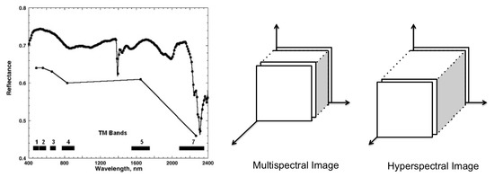
(Figure 1—Left).

Figure 1.

Left

: The wavelength acquisition of spectral bands for multispectral (below) and hyperspectral sampling (above) (taken from

^[9]

Right: a schema of multispectral and hyperspectral images in the spatial-spectral domain.

: a schema of multispectral and hyperspectral images in the spatial-spectral domain.

Having hundreds of narrow and contiguous spectral bands, hyperspectral images (HSI) come with specific challenges intrinsic to their nature that do not exist with multispectral (MSI) and panchromatic images. These challenges include: (1) High-dimensionality of HSI, (2) different types of noise for each band, (3) uncertainty of observed source, and (4) non-linear relations between the captured spectral information

^[10]. The latter is explained to result from the scatterings of surrounding objects during the acquisition process, the different atmospheric and geometric distortions, and the intra-class variability of similar objects.

Despite the mentioned differences in the nature of MSI and HSI, both share a similar 3D cubic-shape structure (Figure 3—Right) and are mostly used for similar purposes. Indeed, the idea behind LULC classification/segmentation relies on the morphological characteristics and material differences of on-ground regions and items, which are respectively retrievable from spatial and spectral information available in both MSI and HSI. Therefore, unlike

. The latter is explained to result from the scatterings of surrounding objects during the acquisition process, the different atmospheric and geometric distortions, and the intra-class variability of similar objects.

^[11] that review methodologies designed for spectral-spatial information fusion for only hyperspectral image classifications, in this review we consider both data types as used in the literature for land cover classifications using deep learning techniques focusing on the spectral and/or spatial characteristics of land cover correlated pixels.

that review methodologies designed for spectral-spatial information fusion for only hyperspectral image classifications, in this review we consider both data types as used in the literature for land cover classifications using deep learning techniques focusing on the spectral and/or spatial characteristics of land cover correlated pixels.

3. Machine Learning for Land Use and Land Cover Classification of Remote Sensing Data

Conventional supervised Land Use and Land Cover (LULC) classification machine learning pipelines usually include four major steps: (1) pre-processing, (2) feature engineering, (3) classifier training and (4) post-processing (Figure 2—top). Each of these stages may be composed of a set of sub-tasks. A good break down of the whole process into its sub-tasks, with an explicit statement of their assumptions, helps to define standalone sub-problems that can be studied independently and have solutions or models that can be incorporated into a LULC pipeline to accomplish the targeted classification/segmentation. Over the last years, with the growing popularity of deep learning as a very powerful tool in solving different types of AI problems, we are witnessing a surge in demand of research to employ deep learning techniques in tackling these sub-problems.

Remotesensing 12 02495 g005 550

Figure 2. The machine learning classification frameworks. The upper one shows the common steps of the conventional approaches, and the lower one shows the modern end-to-end structure. In the end-to-end deep learning structure, the feature engineering is replaced with feature learning as a part of the classifier training phase.

With the increased computational capacity in the new generation of processors, over the last decade, the

The machine learning classification frameworks. The upper one shows the common steps of the conventional approaches, and the lower one shows the modern end-to-end structure. In the end-to-end deep learning structure, the feature engineering is replaced with feature learning as a part of the classifier training phase.

With the increased computational capacity in the new generation of processors, over the last decade, the

end-to-end

deep learning approach received lots of attention from the scientists. The end-to-end learning pipeline—taking the source data as the input-end and the classified map as the output-end—is a modern form of re-designing the process workflow, that is taking advantage of deep learning techniques in solving complex problems. Within the end-to-end deep learning structure, the feature engineering is replaced by

feature learning as a part of the classifier training phase (Figure 2-bottom). In this case, instead of defining the inner steps of the feature engineering phase, the end-to-end architecture generalises the model generation involving feature learning as part of it. Such improved capacity of deep learning has promoted its application on many research works where well-known, off-the-shelf, end-to-end models are directly applied to new data, such as remote sensing. However, there are some open-problems, complexities, and efficiency issues in the end-to-end use of deep learning in LULC classification, that encourages us to adopt a new approach for investigation of the state-of-the-art in deep learning for LULC classification.

as a part of the classifier training phase (Figure 2-bottom). In this case, instead of defining the inner steps of the feature engineering phase, the end-to-end architecture generalises the model generation involving feature learning as part of it. Such improved capacity of deep learning has promoted its application on many research works where well-known, off-the-shelf, end-to-end models are directly applied to new data, such as remote sensing. However, there are some open-problems, complexities, and efficiency issues in the end-to-end use of deep learning in LULC classification, that encourages us to adopt a new approach for investigation of the state-of-the-art in deep learning for LULC classification.

3.1. Deep learning architecture

Deep learning is a group of machine learning techniques that has the capacity to learn a hierarchy of features or representations (the observations or characteristics on which a model is built

^[12]

). Deep learning models are composed of multiple layers such that each layer computes a new data representation from the representation in the previous layers of artificial neurons creating a hierarchy of data abstractions

^[13]

. Convolutional Neural Network (CNNs) are a group of deep learning techniques that are composed of convolution and pooling layers that are usually concluded by a fully connected neural network layer and a proper activation function. CNNs are feedforward neural networks (artificial neural networks wherein no cycle is formed by the connections between its nodes/neurons) that are designed to process the data types composed of multiple arrays (e.g., images, which have layers of 2D-array of pixels)

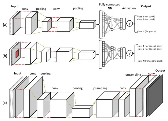
^[13]. Each CNN, as shown in Figure 3, contains multiple stages of convolution and pooling, creating a hierarchy of dependant feature maps.

. Each CNN, as shown in Figure 3, contains multiple stages of convolution and pooling, creating a hierarchy of dependant feature maps.

Figure 3.

An example of convolutional neural network with two layers of convolution and two layers of pooling, for (

) patch level classification, (

) pixel level classification and (

c) an image reconstructive model. The resulting cubes after each layer of convolution and pooling are called feature maps.

) an image reconstructive model. The resulting cubes after each layer of convolution and pooling are called feature maps.

At each layer of convolution, the feature maps are computed as the weighted sum of the previous layer of feature patches, using a filter with a stack of fixed-size kernels, and then pass the result into non-linearity, using an activation function (e.g., ReLU). In such a way, they detect local correlations (fitted in the kernel size), while keeping invariance to the location within the input data array. The pooling layer is used to reduce the dimension of the resulted feature map by calculating the maximum or the average of neighbouring units to create invariance to scaling, small shifts, and distortions. Eventually, the stages of convolution and pooling layers are concluded by a fully connected neural network and an activation function, which are in charge of the classification task within the network.

The process of training a CNN model, using a set of training samples, finds optimised values for the model learnable parameters, by reducing the cost calculated via a

loss function (e.g., Minimum Square Error, Cross Entropy, or Hinge loss). In CNNs, learnable parameters are the weights associated with both convolution layer filters and connections between the neurons in the fully connected neural network. Therefore, the aim of the optimiser (e.g., Stochastic Gradient Descent, RMSprop, or Adam) is not only to train the classifier, but it is also responsible to learn data features by optimizing convolution layers parameters.

(e.g., Minimum Square Error, Cross Entropy, or Hinge loss). In CNNs, learnable parameters are the weights associated with both convolution layer filters and connections between the neurons in the fully connected neural network. Therefore, the aim of the optimiser (e.g., Stochastic Gradient Descent, RMSprop, or Adam) is not only to train the classifier, but it is also responsible to learn data features by optimizing convolution layers parameters.

3.2. End-to-end deep learning challenges

The use of deep learning as an end-to-end approach comes with some complexities and inefficiencies in the processing time. One insight is based on the Wolpert’s “No Free Lunch” (NFL) theorem

^[14]

that refutes the idea of a generalised single machine learning algorithm for all types of problems and data, and underlines the need to check all assumptions and if they are satisfied in our particular problem. Although end-to-end deep learning models have shown a great capacity to generalise well in practice, it is theoretically unclear and is still getting questioned

^{[15][16][17][18]}

. Another issue is that effective use of end-to-end approaches on remote sensing data requires a massive amount of training samples that well cover the output-end’s class distributions. However, due to difficulties in the collection of LULC ground-truth, it is subjected to the issue of the limited number of training samples. Moreover, even if we could find an effective solution to increase the size of training datasets, for example, via unsupervised or semi-supervised learning, the issue of processing efficiency remains. The complexities in the nature of remote sensing data, such as multi-modality, resolution, high-dimensionality, redundancy and noise in data make it even more complex and challenging to model an end-to-end workflow for the LULC classification of remote sensing data. The more complex the model architecture becomes, the more difficult the learning problem gets and it leads to more difficult optimisation problems and dramatically decreases the computational efficiency. Therefore, despite the substantial attempts in applying end-to-end deep learning in LULC classification problems, the challenges of such structure open up the floor for alternative approaches and make the former four-stage machine learning pipeline structure a debatable candidate.

3.3. Four-stage machine learning

Defining the process according to a conventional workflow format makes it easier to shape, customise, and adapt the system to meet the targeted needs and, at the same time, it reduces the model optimisation complexity and computational time of the learning process. Breaking down the assumptions, needs, and targets into a set of sub-tasks, the empirical process of choosing an effective algorithm for each sub-task becomes easier and more diagnosable. Indeed, we can employ deep learning techniques more effectively and transparently to accomplish single sub-tasks of a classical machine learning pipeline with smaller problems to solve. All the solutions and trained models for each sub-task can be then employed in parallel streams or in sequential order at different steps of the conventional workflow.

4. Conclusion

The potentials and challenges of employing deep learning on remote sensing data is shortly addressed and the need for a deeper understating of machine learning as a complex problem is underlined. A complete study that discusses and reviews the state-of-the-art in the field is provided in

In this review, the potentials and challenges of employing deep learning on remote sensing data is shortly addressed and the need for a deeper understating of machine learning as a complex problem is underlined. A complete study that discusses and reviews the state-of-the-art in the field is provided in

^[19]. This study presents also the promising areas in which the implementation of deep learning can be of high potential in the future.

. This study presents also the promising areas in which the implementation of deep learning can be of high potential in the future.

References

Towards a European AI4EO R&I Agenda . ESA. Retrieved 2020-8-17
Tim Newbold; Lawrence N. Hudson; Samantha L. L. Hill; Sara Contu; Igor Lysenko; Rebecca A. Senior; Luca Börger; Dominic J. Bennett; Argyrios Choimes; Ben Collen; et al.Julie DayAdriana De PalmaSandra DíazSusy Echeverría-LondoñoMelanie J. EdgarAnat FeldmanMorgan GaronMichelle L. K. HarrisonTamera AlhusseiniDaniel J. IngramYuval ItescuJens KattgeVictoria KempLucinda KirkpatrickMichael KleyerDavid Laginha Pinto CorreiaCallum D. MartinShai MeiriMaria NovosolovYuan PanHelen R. P. PhillipsDrew W. PurvesAlexandra RobinsonJake SimpsonSean L. TuckEvan WeiherHannah J. WhiteRobert M. EwersGeorgina M. MaceJörn P. W. ScharlemannAndy Purvis Global effects of land use on local terrestrial biodiversity. Nature 2015, 520, 45-50, 10.1038/nature14324.
Peter M. Vitousek; Jane Lubchenco; Jerry M. Melillo; Harold A. Mooney; Human Domination of Earth's Ecosystems. Science 1997, 277, 494-499, 10.1126/science.277.5325.494.
Johannes Feddema; Keith W. Oleson; G. B. Bonan; Linda O. Mearns; Lawrence E. Buja; Gerald A. Meehl; Warren M. Washington; The Importance of Land-Cover Change in Simulating Future Climates. Science 2005, 310, 1674-1678, 10.1126/science.1118160.
Turner, Billie; Richard, H. Moss, and D. L. Skole. Relating Land Use and Global Land-Cover Change; IGBP Report 24, HDP Report 5; International Geosphere-Biosphere Programme: Stockholm, Sweden, 1993.
United Nations Office for Disaster Risk Reduction. Sendai framework for disaster risk reduction 2015–2030. In Proceedings of the 3rd United Nations World Conference on Disaster Risk Reduction (WCDRR), Sendai, Japan, 14–18 March 2015; pp. 14–18.
Zikopoulos, Paul; Eaton, Chris. Understanding Big Data: Analytics for Enterprise Class Hadoop and Streaming Data; McGraw-Hill Osborne Media: New York, NY, USA, 2011.
Xiao Xiang Zhu; Devis Tuia; Lichao Mou; Gui-Song Xia; Liangpei Zhang; Feng Xu; Friedrich Fraundorfer; Deep Learning in Remote Sensing: A Comprehensive Review and List of Resources. IEEE Geoscience and Remote Sensing Magazine 2017, 5, 8-36, 10.1109/mgrs.2017.2762307.
Alexander F.H. Goetz; Three decades of hyperspectral remote sensing of the Earth: A personal view. Remote Sensing of Environment 2009, 113, S5-S16, 10.1016/j.rse.2007.12.014.
Pedram Ghamisi; Emmanuel Maggiori; Shutao Li; Roberto Souza; Yuliya Tarablaka; Gabriele Moser; Andrea De Giorgi; Leyuan Fang; Yushi Chen; Mingmin Chi; et al.Sebastiano B. SerpicoJon Atli Benediktsson New Frontiers in Spectral-Spatial Hyperspectral Image Classification: The Latest Advances Based on Mathematical Morphology, Markov Random Fields, Segmentation, Sparse Representation, and Deep Learning. IEEE Geoscience and Remote Sensing Magazine 2018, 6, 10-43, 10.1109/mgrs.2018.2854840.
Maryam Imani; Hassan Ghassemian; An overview on spectral and spatial information fusion for hyperspectral image classification: Current trends and challenges. Information Fusion 2020, 59, 59-83, 10.1016/j.inffus.2020.01.007.
Removing the Hunch in Data Science with AI-Based Automated Feature Engineering . IBM. Retrieved 2020-8-17
Yann A. LeCun; Yoshua Bengio; Geoffrey Hinton; Deep learning. Nature 2015, 521, 436-444, 10.1038/nature14539 10.1038/nature14539.
David H. Wolpert; The Lack of A Priori Distinctions Between Learning Algorithms. Neural Computation 1996, 8, 1341-1390, 10.1162/neco.1996.8.7.1341.
Zhang, Chiyuan; Bengio, Samy; Hardt, Moritz; Recht, Benjamin; Vinyals, Oriol; Understanding deep learning requires rethinking generalization. arXiv 2016, arXiv:1611.03530.
Kawaguchi, Kenji; Kaelbling, Leslie Pack; Bengio, Yoshua; Generalization in deep learning. arXiv 2017, arXiv:1710.05468.
Andrew M Saxe; Yamini Bansal; Joel Dapello; Madhu Advani; Artemy Kolchinsky; Brendan D Tracey; David D Cox; On the information bottleneck theory of deep learning. Journal of Statistical Mechanics: Theory and Experiment 2019, 2019, 124020, 10.1088/1742-5468/ab3985.
Dinh, Laurent, Razvan Pascanu; Bengio, Samy, Bengio, Yoshua; Sharp Minima Can Generalize For Deep Nets. In Proceedings of the 34th International Conference on Machine Learning (ICML), Sydney, Australia, 2017, 1019–1028.
Ava Vali; Sara Comai; Matteo Matteucci; Deep Learning for Land Use and Land Cover Classification based on Hyperspectral and Multispectral Earth Observation Data: A Review. Remote Sensing 2020, 12, 2495, 10.3390/rs12152495.