Magnetic Guiding with Permanent Magnets

Magnetic Guiding with Permanent Magnets: Comparison

Please note this is a comparison between Version 1 by Peter Blümler and Version 8 by Lindsay Dong.

Magnetic guidance is understood as a remote, untethered and contact-free control of the movements of an object via magnetic interactions. The movements should happen on arbitrary trajectories inside a container caused by an external device.

In Tthis review the conceptidea of remote magnetic guiding is developed from the underlying physics of a concept that allows for bijective force generation over the inner volume of magnet systems. This concept can equally be implemented by electro- or permanent magnets.

steering
magnetic force
magnetic drug targeting (MDT)
nanoparticle
SPIO
ferrofluid
superparamagnetic
ferromagnetic
Halbach magnets
dipole
quadrupole
cells
micro-robots
endoscopic capsules
magnetic resonance imaging
MRI

1. History/Problem

Examples:

Magnetic guiding has been an established technique since 1897^[1], when Ferdinand Braun invented magnetic guidance of charged particles (electrons or ions) by cathode ray tubes where the electrons are emitted from a cathode into an evacuated tube, accelerated by an anode, and deflected by magnetic fields (used en masse in analogue oscilloscopes and television screens). The magnetic deflection is based on the Lorentz force FL=qv × B, which is perpendicular to the direction of the magnetic flux density B and the flight direction of the particles with charge q and velocity v. However, the situation is very different if an electrically neutral paramagnetic material is exposed to magnetic fields. The force is then the gradient (∇ = [∂/∂x, ∂/∂y, ∂/∂z]) of the magnetic field acting on the object with a magnetic moment m,

So what hapTypens to a small paramagnetic object in an inhomogeneous magnetic field? It is hard to imagine that an object that should be guided through space is not freely movable (at least in two dimensions). If the object has an intrinsic fixed direction of m (e.g., remal exanent magnetization), it is rotated by the magnetic torque,

Until the cross-product becomes zero or m is parallel to B. If the object has initially (at B = 0 ) no preferred direction of m, the actual field will magnetize it (orient the electron spins) along B. Either way, as a result, m points along B, which is very unfortunate with respect to guiding, because the dot-product in Fm = (m · ∇) B will lose its sign for two parallel vectors and the material will always move towards higher magnetic fields (cf. Figure 1a,b). . This is an everyday observation, as e.g., paper clips are attracted equally by the north and south pole of a permanent magnet. For steering this is like using a clipper without a sail. Almost independently of what one tries with the rudder, the boat will go to where the winds or currents move it. In electrodynamics, this is also known as Earnshaw’s theorem^[2], and it is the reason why permanent magnets were originally not considered as being useful for magnetic guidance, because as their name suggests they are permanent and cannot be switched on or off.

Figure 1. Illustration of the suggested guiding principle. A small magnetizable sphere serves as the object to be guided by a large deflecting bar magnet. The colors indicate the magnitude of the local magnetic flux density (see color bars on the left, Bmax in (a,b) is roughly a quarter of that in (c,d)). The black lines are field lines. A zoom of the region around the object is shown on the inserts. The top rows (a,b) just show the field generated by the deflection magnet, while in (c,d) a strong and homogeneous field is superimposed to the scenario above. The difference between the columns is the orientation (south- and north-pole) of the deflection magnet. (a,b) Changing the magnet’s orientation has no effect on the movement of the object (white arrow), because the object is magnetized in opposite directions as well and just moves to the highest flux density. The additional homogeneous field in (c,d) essentially keeps the magnetization direction of the object along its horizontal direction. The field of the deflecting magnet now causes the opposite magnetic “landscape” around the object and hence moves in opposite directions. The data were generated using FEMM but should serve for illustration purposes only.

2. Solution

Now the question arises why guiding charged particles is so straightforward, while it is so difficult to control the collective spin of electrons in materials maof such magnetically? The reason is the bijective direction (v) guided of the electron beam, which is just slightly deflected by steering fields. This suggests that a preferred direction would also be beneficial for steering paramagnetic objects. This is tantamount to a magnetic field that just orients (polarizes) the particles without exerting a force on them. For static magnetic fields, this request can be fulfilled by applying a strong but homogeneous magnetic flux density, Bhom, which magnetizes the object along its direction. An additional, small, and spatially-dependent steering or deflecting field can then act as a perturbation but with full directional control (cf. Figure 1c,d). Ideally, thjects are endoscopic capsules for is deflecting field will have a linear spatial dependence, i.e., a constant gradient (The fact that G is a tensor is ignored for the moment), ∇ B = G , and the total spection ofield in such an experiment is then

Withthe the reasonable assumption that there is no strong spatial variation of the magnetic moment over the sample, one could conclude that Fm = mG (because ∇Bhom = 0). Undeastr certain limits this is correct, but unfortunately magnetism is not quite that simple. Things become a bit more complicated due to Maxwell’s (or Gauss’) law

Heintestince, there cannot be a single gradient field at any point. Either the field has to be homogeneous or the sum of all its spatial derivatives have to cancel. For the simple case of a perfect quadrupolar field , this could be for instance ∂Bx /∂x = +G and ∂By /∂y = -G consequently the last equation then dictates ∂Bz /∂z = 0. Then a more detailed representation of B(r) will be

The deflecting field is written here in the most general form as a gradient tensor (G). As discussed above, the magnetic moment of an object at r = [x, y, z]^Twill be oriented parallel to B(r) (with unit vector eB)

The last approximation was already motivated in the discussion of Figure 1 and is the origin of bijection, namely that the homogeneous field must be much stronger than the local deflection field, so that its tensorial properties can be reduced to a vector via projection. The condition for this prerequisite is then^[3]

It is instructive to continue with this assumption to approximate the magnetic force

Or more generally only the field component of the deflection field, which is parallel to Bhom, determines the direction and amplitude of the magnetic force. It is a very beneficial feature of this concept that there is no spatial dependence of the force vector in last equation, hence the guiding force is homogeneous or constant over that region where Bhom >> Gr is fulfilled . This is an important issue because other systems which guide an object by moving permanent magnets around the outside of the container (e.g.^[4]) or use electromagnets on opposing ends of the container, also have to consider the non-linear drop of the magnetic field with distance (depending on their dimensions, the far-field of permanent magnets drops with an exponent between −2 and −3, and hence the force with −3 to −4). This can extremely complicate the control because the position of the object has to be known precisely to estimate speed and direction of motion. This is a problem that does not exist in the presented concept. Additionally, the movements are also not limited to the direction of B.

3. Realisation with permanent magnets

The descl tract or superibed concept is easy to realize by so-called Halbach cylinders^[3][5], the hoaramogeneous field will be generated by a Halbach dipole (see Fig. 2a) while the constant gradients can readily be provided by a Halbach quadrupole (see Fig. 2b). The first advantage of such Halbach cylinders is that they provide ideal homogeneous and graded fields (as are assumed for eq. (8)) with simple geometric relations to calculate their field

where Ri is gnetic nanoparthe inner and Ro the outer radius of the hollow cylinders and BR [T] is the remanence of the used permanent magnet material.

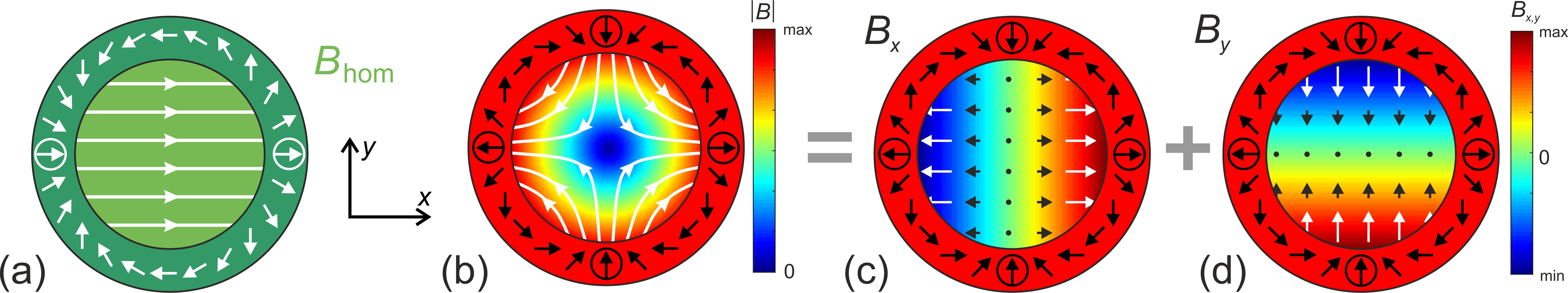
Figure 2. Sketch of ideal Halbach cylinders: (a) inner dipole with a homocles suggeneous field of strength, Bhom along the x-axis. (b) inner quadrupole with a circular modulus field which can be decomposed into a two linear field components Bx = Gx in (c) and By = -Gy in (d). The hollow cylinders consist of permanent magnet material with continuously changing magnetization direction (arrows). The poles are encircled. In (a) and (b) the magnetic field is represented by field lines, while in (c) and (d) the arrows are field vectors (the different colors are only for better contrast). Note that the magnetic fields are only inside the hollow cylinders and that there are no stray fields.

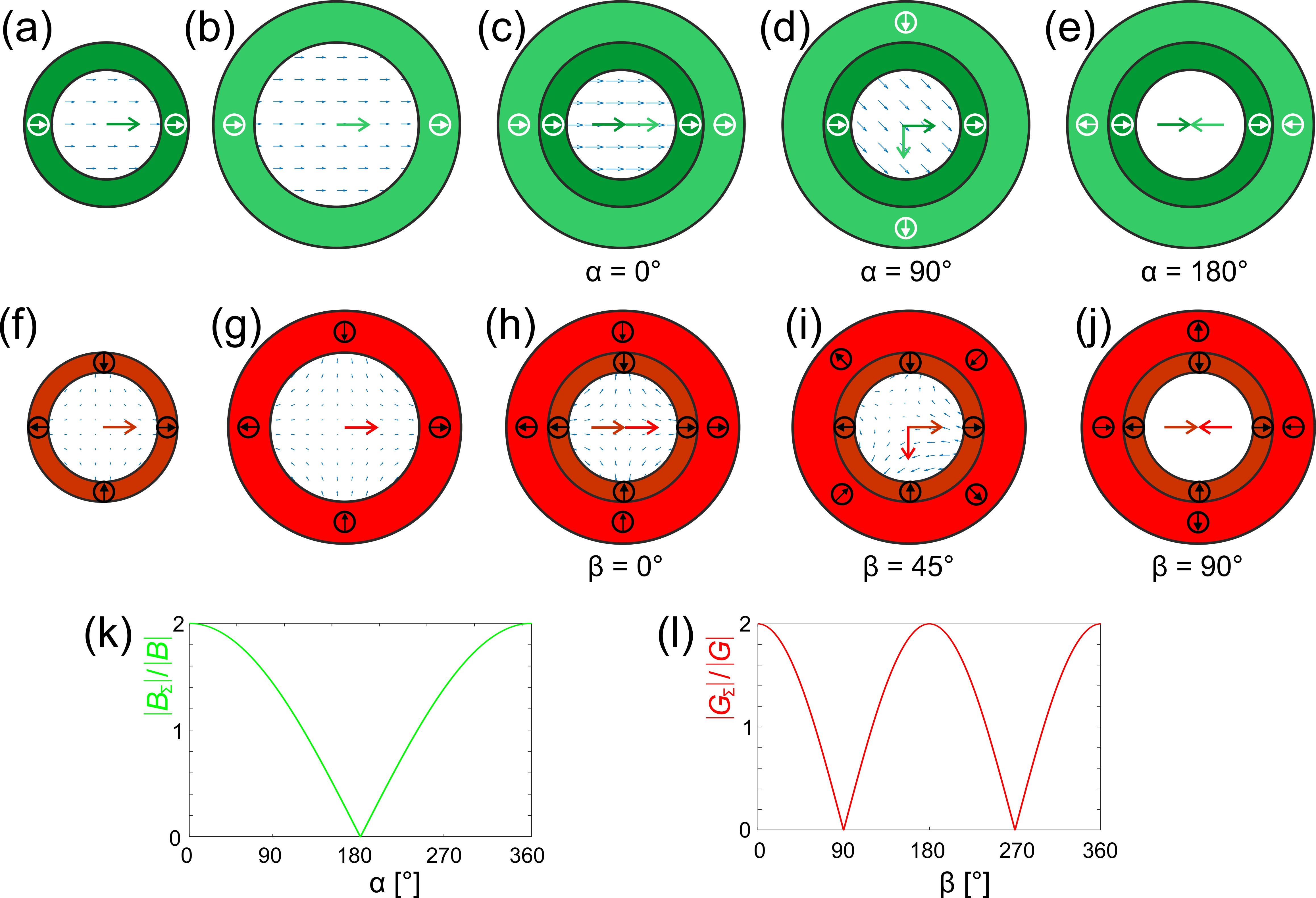
The second great adted for local therapy, which therefore havantage is the absence of stray fields, so that they are “no magnets” when approached from the outside. Therefore, the cylinders can be concentrically arranged or nested and mutually rotated without much torque^[6]. If twto be moved thro Halbach cylinders of the same type are nested and the geometries are chosen such that they both produce the same field or gradient strength, their combined field can then be varied between zero and twice the value of a single cylinder. This allows to scale the field or force or eventually even switch it off by simple mechanical rotation. This principle is illustrated in Figgh blood vessels. 3.

reviews:

magnetically guided medical devices ^[1][2]^[3]

miniature robots^[4]

nanoparticles in microfluidics and nanomechanics^[5] for drug delivery^[6][7][8]

hyperthermia, and alternative local magnetic therapeutic effects^[9][10]

tissue engineering^[11][12]^[13]

as well as magnet systems for this purpose^[14]

monograph^[15] treating most of these topics

Concept:

Magnetic guiding has been an established technique since 1897^[16], when Ferdinand Braun invented magnetic guidance of charged particles (electrons or ions) by cathode ray tubes where the electrons are emitted from a cathode into an evacuated tube, accelerated by an anode, and deflected by magnetic fields (used en masse in analogue oscilloscopes and television screens). The magnetic deflection is based on the Lorentz force \vec{F}_L = q \vec{v} \times \vec{B}

{\overset{⇀}{F}}_{L} = q \overset{⇀}{v} \times \overset{⇀}{B},

which is perpendicular to the direction of the magnetic flux density \vec{B} and the flight direction of the particles with charge q and velocity \vec{v} . However, the situation is very different if an electrically neutral paramagnetic material is exposed to magnetic fields. The force is then the gradient (\vec{\nabla} = [\partial/\partial x,\partial/\partial y,\partial/\partial z]) of the magnetic field acting on the object with a magnetic moment \vec{m}

\vec{F}_m = \vec{\nabla} (\vec{m} \cdot \vec{B}) \approx (\vec{m} \cdot \vec{\nabla}) \vec{B} (1)   The right simplified term is usually correct for the applications discussed here, however, it is not generally the case. Particularly, it assumes that m is not dependent on B , which depends on the material and the range of B .

So what happens to a small paramagnetic object in an inhomogeneous magnetic field? It is hard to imagine that an object that should be guided through space is not freely movable (at least in two dimensions). If the object has an intrinsic fixed direction of \vec{m} (e.g., remanent magnetization), it is rotated by the magnetic torque

\vec{\tau}_m = \vec{m} \times \vec{B},

(2)

until the cross-product becomes zero or \vec{m} is parallel to \vec{B} . If the object has initially (at B=0 ) no preferred direction of \vec{m} , the actual field will magnetize it (orient the electron spins) along \vec{B} . Either way, as a result, \vec{m} points along \vec{B} , which is very unfortunate with respect to guiding, because the dot-product in Equation (1) will lose its sign for two parallel vectors and the material will always move towards higher magnetic fields (cf.

Figure 31

a,b). This is an everyday observation, as e.g., paper clips are attracted equally by the north and south pole of a permanent magnet. For steering this is like using a clipper without a sail. Almost independently of what one tries with the rudder, the boat will go to where the winds or currents move it. In electrodynamics, this is also known as Earnshaw’s theorem^[17], and it is the reason why permanent magnets were originally not considered as being useful for magnetic guidance, because as their name suggests they are permanent and cannot be switched on or off.

Figure 1.

Coaxial arrangement and rotation of Halbach dipoles (green, upper row) and quadrupoles (red, lower row): (

Illustration of the suggested guiding principle. A small magnetizable sphere serves as the object to be guided by a large deflecting bar magnet. The colors indicate the magnitude of the local magnetic flux density (see color bars on the left, B_{max} in (a,b) is roughly a quarter of that in (c,d)). The black lines are field lines. A zoom of the region around the object is shown on the inserts. The top rows (

a) and (

b) two Halbach dipoles which produce the same field strength, B (central green arrow); are coaxially nested in (

) just show the field generated by the deflection magnet, while in (

c-e) and the outer one is rotated by an angle α. The resulting field is also illustrated by B-arrows. (

,d) a strong and homogeneous field is superimposed to the scenario above. The difference between the columns is the orientation (south- and north-pole) of the deflection magnet. (a,b) Changing the magnet’s orientation has no effect on the movement of the object (white arrow), because the object is magnetized in opposite directions as well and just moves to the highest flux density. The additional homogeneous field in (

c) For α = 0° the fields are parallel and the two dipole fields add to 2B . (

d) For α = 90° the fields are orthogonal and the two dipole field vectors add to √2|B| at an angle of 45°. (

) essentially keeps the magnetization direction of the object along its horizontal direction. The field of the deflecting magnet now causes the opposite magnetic “landscape” around the object and hence moves in opposite directions. The data were generated using FEMM but should serve for illustration purposes only.

Now the question arises why guiding charged particles is so straightforward, while it is so difficult to control the collective spin of electrons in materials magnetically? The reason is the bijective direction ( \vec{v} ) of the electron beam, which is just slightly deflected by steering fields. This suggests that a preferred direction would also be beneficial for steering paramagnetic objects. This is tantamount to a magnetic field that just orients (polarizes) the particles without exerting a force on them. For static magnetic fields, this request can be fulfilled by applying a strong but homogeneous magnetic flux density, B_{hom} , which magnetizes the object along its direction. An additional, small, and spatially-dependent steering or deflecting field can then act as a perturbation but with full directional control (cf. Figure

) For α = 180° the fields are antiparallel and cancel each other. An analog presentation is shown in (f-g) for two nested quadrupoles which produce the same field gradient (i.e. the derivative of the field! The red arrow shows the horizontal component only). (h-j) Same representation as above. Note that the gradient rotates at twice the angle of the quadrupole

1c,d). Ideally, this deflecting field will have a linear spatial dependence, i.e., a constant gradient (The fact that \overline{\overline{G}} is a tensor is ignored for the moment), \vec{\nabla}\vec{B}=G , and the total field in such an experiment is then

\vec{B}(\vec{r})=\vec{B}_{hom}+G\vec{r}.

(3)

With the reasonable assumption that there is no strong spatial variation of the magnetic moment over the sample, one could conclude that F_m=mG (because

\overset{⇀}{\nabla} {\overset{⇀}{B}}_{hom} = 0

). Under certain limits this is correct, but unfortunately magnetism is not quite that simple. Things become a bit more complicated due to Maxwell’s (or Gauss’) law

\vec{\nabla}\cdot\vec{B}=\frac{\partial B_x}{\partial x}+\frac{\partial B_y}{\partial y}+\frac{\partial B_z}{\partial z} = 0 .(4) Hence, there cannot be a single gradient field at any point. Either the field has to be homogeneous or the sum of all its spatial derivatives have to cancel. For the simple case of a perfect quadrupolar field , this could be for instance  \partial B_x/\partial x = +G and \partial B_y/\partial y = -G consequently Equation (4) then dictates \partial B_z/\partial z = 0 . Then a more detailed representation of Equation (3) will be

\begin{align*}\vec{B}(\vec{r}) &= \begin{bmatrix} B_x(x,y,z) \\B_y(x,y,z)\\B_z(x,y,z) \end{bmatrix} =\vec{B}_{hom} + G\vec{r} \\ &= B_{hom}\begin{bmatrix}1\\0\\0 \end{bmatrix}+G\begin{bmatrix}1&0&0\\0&-1&0\\0&0&0 \end{bmatrix} \begin{bmatrix}x\\y\\z \end{bmatrix} =\begin{bmatrix}B_{hom}+Gx\\-Gy\\0 \end{bmatrix} \end{align*} (5)

The deflecting field is written here in the most general form as a gradient tensor ( \overline{\overline{G}} ). As discussed above, the magnetic moment of an object at \vec{r}=[x,y,z]^T will be oriented parallel to \vec{B}(\vec{r}) (with unit vector \hat{e}_B )

\begin{align*} \vec{m}(x,y,z) &= \big| \vec{m} \big| \hat{e}_B = \big| \vec{m} \big| \frac {\vec{B}} {\big|\vec{B}\big|} \\ &=\frac {\big| \vec{m} \big|} {\sqrt{(B_{hom}+Gx)^2+G^2y^2}} \begin{bmatrix}B_{hom}+Gx\\-Gy\\0 \end{bmatrix} \stackrel{B_{hom} \gg Gr}{\approx} \big| \vec{m}\big| \begin{bmatrix}1\\0\\0 \end{bmatrix} \end{align*} (6) The last approximation was already motivated in the discussion of Figure 1 and is the origin of bijection, namely that the homogeneous field must be much stronger than the local deflection field, so that its tensorial properties can be reduced to a vector via projection. The condition for this prerequisite is then

\big|\vec{B}_{hom}\big| \gg \big|\vec{\nabla}\vec{B} \big| \big|\vec{r} \big| (7)   A full treatment[18] will follow but to clarify the concept, it is instructive to continue with the approximation from Equation (6). Then the magnetic force in Equation (1) simplifies to

\begin{align*} \vec{F}_m(x,y,z) & = ( \vec{m} \vec{\nabla})\vec{B} \approx \big| \vec{m} \big| \frac {\partial} {\partial x} \begin{bmatrix}B_{hom}+Gx\\-Gy\\0 \end{bmatrix} \\ & =\big| \vec{m} \big| G \hat{e}_x, \end{align*} (8)     or more generally only the field component of the deflection field, which is parallel to \vec{B}_{hom} , determines the direction and amplitude of the magnetic force. It is a very beneficial feature of this concept that there is no spatial dependence of the force vector in Equation (8), hence the guiding force is homogeneous or constant over that region where Equation (7) is fulfilled (cf. also Figure 5). This is an important issue because other systems which guide an object by moving permanent magnets around the outside of the container (e.g.

^[319]. (k)

) or use electromagnets on opposing ends of the container, also have to consider the non-linear drop of the magnetic field with distance (depending on their dimensions, the far-field of permanent magnets drops with an exponent between −2 and −3, and hence the force with −3 to −4). This can extremely complicate the control because the position of the object has to be known precisely to estimate speed and direction of motion. This is a problem that does not exist in the presented concept. Additionally, the movements are also not limited to the direction of \vec{B} .

The angular dependence of the combined field of both dipoles, BΣ = 2|B||cos(α/2)|,s (l) Angular dependence of the gradient strength of the two quadrupoles GΣ = 2|G||cosα|.

If the previous example is realized by a Halbach dipole and a Halbach quadrupole and the quadrupole is rotated by an angle α relative to the dipole, the magnetic field in such a structure is (cf.Fig. 3l)

Using the same arguments as before (i.e. that the field component which is not along BD [there. By] can be ignored for BD >> Gr) the magnetic force is then given by

This means that the magnetic force has a constant strength of |m|GQ and rotates with 2α over the entire von alume where the prerequisite BD >> Gr is fulfilled.

In order to completely control the movements of such a guided object, not only the direction but also the amplitude of the force must be controlled. This can easily be done by using a second quadrupole, ideally of a size that produces the same gradient strength in the internal volume as already provided by the first quadrupole. If the direction of the force shall be determined by α and shall not be altered by scaling the force, one quadrupole must be rotated by an angle (α+β/2) and the other by (α-β/2). Hence, generating a force

Such a system allows complete control in two dimensions as demonstrated in this video .

4. Examples/Further reading

Examples:

Typical eexamples of such magnetically guided objects are endoscopic capsules for inspection of the gastrointestinal tract or superparamagnetic nanoparticles suggested for local therapy, which therefore have to be moved through blood vessels.ains:

Reviews:

How such magnetic fields (equation (8)) can be generated using permanent magnets with adjustable fields.

How the magnetic force deviates from being constant if equation (7) is violated.

How the velocity of objects can be calculated from the magnetic force.

Possible 3D designs of such guiding machines

Localization of the guided object via MRI or MPI

Applications

Seven appendices contain mathematical details and practical considerations for designing and constructing such devices

magnetically guided medical devices ^[7][8]^[9]

miniature robots ^[10]

nanoparticles in microfluidics and nanomechanics ^[11] for drug delivery ^[12][13][14]

hyperthermia, and alternative local magnetic therapeutic effects ^[15][16]

tissue engineering ^[17][18]^[19]

as well as magnet systems for this purpose ^[20]

monograph ^[21] treating most of these topics

References

Braun, F.; Ueber ein Verfahren zur Demonstration und zum Studium des zeitlichen Verlaufes variabler Ströme. AnnSliker, L.; Ciuti, G.; Rentschler, M.; Menciassi, A.; Magnetically driven medical devices: A review. Expert Rev. PhysMed. Chem. Devices 201897, 60, 552, https://doi.org/10.1002/andp.18972960313.5, 12, 737, https://doi.org/10.1586/17434440.2015.1080120.
Earnshaw, S.; On the nature of the molecular forces which regulate the constitution of the luminiferous ether. TraRivas, H.; Robles, I.; Riquelme, F.; Vivanco, M.; Jimenez, J.; Marinkovic, B.; Uribe, M.; Magnetic surgery: Results from first prospective clinical trial in 50 patients. Anns. Camb. Philos. SocSurg. 201842, , 267, 97., 88, https://doi.org/10.1097/SLA.0000000000002045.
Baun, O.; Blümler, P.; Permanent magnet system to guide superparamagnetic particles. JLi, Y.; Sun, H.; Yan, X.P.; Wang, S.P.; Dong, D.H.; Liu, X.M.; Wang, B.; Su, M.S.; Lv, Y.; Magnetic compression anastomosis for the treatment of benign biliary strictures: A clinical study from China.. Surg. MagEn. Magn. Materdosc. Other Interv. Tech. 202017, , 3439, 294, https://doi.org/10.1016/j.jmmm.2017.05.001., 2541, https://doi.org/10.1007/s00464-019-07063-8.
Carpi, F.; Kastelein, N.; Talcott, M.; Pappone, C.; Magnetically controllable gastrointestinal steering of video capsules. Yang, Z.; Zhang, L.; Magnetic actuation systems for miniature robots: A review. . Adv. IEEE Trans. Biomedtell. Syst. Eng. 202011, 5, 200008, 231, https:\\doi.org\10.1109/TBME.2010.2087332.2, 1, https://doi.org/10.1002/aisy.202000082.
Blümler, P.; Casanova, F.. Hardware Developments: Halbach Magnet Arrays; Johns, M.L.; Fridjonsson, E.O., Vogt, S. J.; Haber, A., Eds.; The Royal Society of Chemistry: Cambridge, UK, 2016; pp. 133.Cao, Q.L.; Fan, Q.; Chen, Q.; Liu, C.T.; Han, X.T.; Li, L.; Recent advances in manipulation of micro- and nano-objects with magnetic fields at small scales. Mater. Horiz. 2020, 7, 638, DOI https://doi.org/10.1039/C9MH00714H.
Leupold, H.A.; Tilak, A.S.; Potenziani II, E.; Adjustable multi-Tesla permanent magnet field sources. IEEELiu, Y.L.; Chen, D.; Shang, P.; Yin, D.C.; A review of magnet systems for targeted drug delivery. J. TraConsactions on Mag¬ntrol. Releasetics 201993, , 3029, 2902, https://doi.org/10.1109/20.281092., 90, https://doi.org/10.1016/j.jconrel.2019.03.031.
Sliker, L.; Ciuti, G.; Rentschler, M.; Menciassi, A.; Magnetically driven medical devices: A review. ExpeShapiro, B.; Kulkarni, S.; Nacev, A.; Muro, S.; Stepanov, P.Y.; Weinberg, I.N.; Open challenges in magnetic drug targeting. Wirt Rev. Med. Devices s Nanomed. Nanobiotechnol. 2015, 12, 737, https://doi.org/10.1586/17434440.2015.1080120., 7, 446, https://doi.org/10.1002/wnan.1311.
Rivas, H.; Robles, I.; Riquelme, F.; Vivanco, M.; Jimenez, J.; Marinkovic, B.; Uribe, M.; Magnetic surgery: Results from first prospective clinical trial in 50 patients. Ann. Surg. 2018, 267, 88, https://doi.org/10.1097/SLA.0000000000002045.Komaee, A.; Lee, R.; Nacev, A.; Probst, R.; Sarwar, A.; Depireux, D.A.; Dormer, K.J.; Rutel, I.; Shapiro, B.. Putting Therapeutic Nanoparticles Where They Need to Go by Magnet Systems Design and Control; Thanh T.K., Eds.; CRC Press: Boca Raton FL, USA, 2012; pp. 419.
Li, Y.; Sun, H.; Yan, X.P.; Wang, S.P.; Dong, D.H.; Liu, X.M.; Wang, B.; Su, M.S.; Lv, Y.; Magnetic compression anastomosis for the treatment of benign biliary strictures: A clinical study from China.. Surg. EndosDay, N.B.; Wixson, W.C.; Shields IV, C.W.; Magnetic systems for cancer immunotherapy. Ac.ta Other Interv. Tech. Pharm. Sin. B 2020, 34, 2541, https://doi.org/10.1007/s00464-019-07063-8.1, 11, 2172, https://doi.org/10.1016/j.apsb.2021.03.023.
Yang, Z.; Zhang, L.; Magnetic actuation systems for miniature robots: A review. . AdvPesqueira, T.; Costa-Almeida, R.; Gomes, M.E.; Magnetotherapy: The quest for tendon regeneration. J. IntCell. SystPhysiol. 2020, 18, 2000082, 1, https://doi.org/10.1002/aisy.202000082.33, 6395, https://doi.org/10.1002/jcp.26637.
Cao, Q.L.; Fan, Q.; Chen, Q.; Liu, C.T.; Han, X.T.; Li, L.; Recent advances in manipulation of micro- and nano-objects with magnetic fields at small scales. MaterParfenov, V.A.; Khesuani, Y.D.; Petrov, S.V.; Karalkin, P.A.; Koudan, E.V.; Nezhurina, E.K.; Pereira, F.; Krokhmal, A.A.; Gryadunova, A.A.; Bulanova, E.A.; et al.et al. Magnetic levitational bioassembly of 3D tissue construct in space. Sci. HorizAdv. 2020, 7, 638, DOI https://doi.org/10.1039/C9MH00714H., 6, eaba4174, https://doi.org/10.1126/sciadv.aba4174.
Liu, Y.L.; Chen, D.; Shang, P.; Yin, D.C.; A review of magnet systems for targeted drug delivery. JGoranov, V.; Shelyakova, T.; De Santis, R.; Haranava, Y.; Makhaniok, A.; Gloria, A.; Tampieri, A.; Russo, A.; Kon, E.; Marcacci, M.; et al.et al. 3D patterning of cells in magnetic scaffolds for tissue engineering. Sci. ControlRep. Release 202019, 3, 102, 90, https://doi.org/10.1016/j.jconrel.2019.03.031., 1, https://doi.org/10.1038/s41598-020-58738-5.
Shapiro, B.; Kulkarni, S.; Nacev, A.; Muro, S.; Stepanov, P.Y.; Weinberg, I.N.; Open challenges in magnetic drug targeting. WiresVanecek, V.; Zablotskii, V.; Forostyak, S.; Ruzicka, J.; Herynek, V.; Babic, M.; Jendelova, P.; Kubinova, S.; Dejneka, A.; Sykova, E.; et al. Highly efficient magnetic targeting of mesenchymal stem cells in spinal cord injury. Int. J. Nanomed. Nanobiotechnol. 2015, 2, 7, 446, https://doi.org/10.1002/wnan.1311., 3719, https://doi.org/10.2147/IJN.S32824.
Komaee, A.; Lee, R.; Nacev, A.; Probst, R.; Sarwar, A.; Depireux, D.A.; Dormer, K.J.; Rutel, I.; Shapiro, B.. Putting Therapeutic Nanoparticles Where They Need to Go by Magnet Systems Design and Control; Thanh T.K., Eds.; CRC Press: Boca Raton FL, USA, 2012; pp. 419.Schuerle, S.; Erni, S.; Flink, M.; Kratochvil, B.E.; Nelson, B.J.; Three-dimensional magnetic manipulation of micro- and nanostructures for applications in life sciences. IEEE Trans. Magn. 2013, 49, 321, https:\\doi.org\10.1109/TMAG.2012.2224693.
Day, N.B.; Wixson, W.C.; Shields IV, C.W.; Magnetic systems for cancer immunotherapy. Acta Pharm. Sin. B 2021, 11, 2172, https://doi.org/10.1016/j.apsb.2021.03.023.Andrä, W.; Nowak, H. . Magnetism in Medicine: A Handbook; Wiley-VCH: Weinheim, Germany, 2007; pp. 630.
Pesqueira, T.; Costa-Almeida, R.; Gomes, M.E.; Magnetotherapy: The quest for tendon regeneration. JBraun, F.; Ueber ein Verfahren zur Demonstration und zum Studium des zeitlichen Verlaufes variabler Ströme. Ann. Cell. Physiol. 20Chem. 18, 233, 6395, https://doi.org/10.1002/jcp.26637.97, 60, 552, https://doi.org/10.1002/andp.18972960313.
Parfenov, V.A.; Khesuani, Y.D.; Petrov, S.V.; Karalkin, P.A.; Koudan, E.V.; Nezhurina, E.K.; Pereira, F.; Krokhmal, A.A.; Gryadunova, A.A.; Bulanova, E.A.; et al.et al. Magnetic levitational bioassembly of 3D tissue construct in space. ScEarnshaw, S.; On the nature of the molecular forces which regulate the constitution of the luminiferous ether. Trans. Camb. Philos. AdvSoc. 1842020, 6, eaba4174, https://doi.org/10.1126/sciadv.aba4174., 7, 97.
Goranov, V.; Shelyakova, T.; De Santis, R.; Haranava, Y.; Makhaniok, A.; Gloria, A.; Tampieri, A.; Russo, A.; Kon, E.; Marcacci, M.; et al.et al. 3D patterning of cells in magnetic scaffolds for tissue engineering. SciBaun, O.; Blümler, P.; Permanent magnet system to guide superparamagnetic particles. J. Magn. Magn. RMatepr. 2020, 10, 1, https://doi.org/10.1038/s41598-020-58738-5.17, 439, 294, https://doi.org/10.1016/j.jmmm.2017.05.001.
Vanecek, V.; Zablotskii, V.; Forostyak, S.; Ruzicka, J.; Herynek, V.; Babic, M.; Jendelova, P.; Kubinova, S.; Dejneka, A.; Sykova, E.; et al. Highly efficient magnetic targeting of mesenchymal stem cells in spinal cord injury. Carpi, F.; Kastelein, N.; Talcott, M.; Pappone, C.; Magnetically controllable gastrointestinal steering of video capsules. IEEE Trant. J. Nans. Biomed. Eng. 20112, 7, 3719, https://doi.org/10.2147/IJN.S32824., 58, 231, https:\\doi.org\10.1109/TBME.2010.2087332.
Schuerle, S.; Erni, S.; Flink, M.; Kratochvil, B.E.; Nelson, B.J.; Three-dimensional magnetic manipulation of micro- and nanostructures for applications in life sciences. IEEE Trans. Magn. 2013, 49, 321, https:\\doi.org\10.1109/TMAG.2012.2224693.
Andrä, W.; Nowak, H. . Magnetism in Medicine: A Handbook; Wiley-VCH: Weinheim, Germany, 2007; pp. 630.
Blümler, P.; Magnetic Guiding with Permanent Magnets: Concept, Realization and Applications to Nanoparticles and Cells. cells 2021, 10, 2708, https://doi.org/10.3390/cells10102708 .

1. History/Problem

Examples:

2. Solution

3. Realisation with permanent magnets

Concept:

4. Examples/Further reading

Examples:

Reviews:

Further reading:

References