AI-Assisted Design-on-Simulation for Life Prediction

AI-Assisted Design-on-Simulation for Life Prediction: Comparison

Please note this is a comparison between Version 1 by Kuo-Ning Chiang and Version 2 by Lindsay Dong.

Many researchers have adopted the finite-element-based design-on-simulation (DoS) technology for the reliability assessment of electronic packaging. DoS technology can effectively shorten the design cycle, reduce costs, and effectively optimize the packaging structure. However, the simulation analysis results are highly dependent on the individual researcher and are usually inconsistent between them. Artificial intelligence (AI) can help researchers avoid the shortcomings of the human factor.

FEM simulation
WLP
AI
machine learning
ANN
RNN
SVR
KRR
KNN
RF
regression model

1. Introduction

Electronics packaging plays an important role in the semiconductor industry. Currently, the mainstream electronic packaging structures include heterogeneous packaging, 3D packaging, system-in-packaging (SiP), fan-out (FO) packaging, and wafer-level packaging ^{[1][2][3][4][5][6][7][8]}[1,2,3,4,5,6,7,8]. With the increasing complexity of packaging structures, manufacturing reliability test vehicles, and conducting ATCT experiments have become time-consuming and very expensive processes, the design-on-experiment (DoE) methodology for packaging design is becoming infeasible. As a result of the wide adoption of finite element analysis ^{[9][10][11][12][13][14][15]}[9,10,11,12,13,14,15], accelerated thermal cycling tests are reduced significantly in the semiconductor industry, and package development time and cost are reduced as well. In a 3D WLP model, Liu [16] applied the Coffin–Manson life prediction empirical model to predict the reliability life of a solder joint within an accurate range. However, the results of finite element simulations are highly dependent on the mesh size, and there is no guideline to help researchers address this issue. Therefore, Chiang et al. [17] proposed the concept of “volume-weighted averaging” to determine the local strain, especially in critical areas. Tsou [18] successfully predicted packaging reliability through finite element simulation with a fixed mesh size in the critical area of the WLP structure. However, the results of simulation analysis are highly dependent on the individual researcher, and the results are usually inconsistent between simulations. In order to overcome this problem, the present work comparatively reviews an artificial intelligence (AI) approach in which electronic packaging design using a machine learning algorithm ^[19][20][19,20]. The use of machine learning for the analysis of electronic packaging reliability is the best way to obtain a reliable prediction result and meet the time-to-market demand.

2. Finite Element Method for WLP

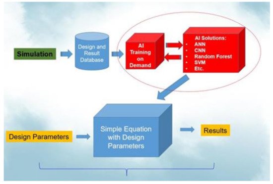
If the simulation consistently predicts the result of the experiment ^[21][52], then the simulation is an experiment; the experimental work can be replaced by a validated simulation procedure to create a large database for AI training and obtain a small and accurate AI model for reliability life cycles prediction. Once we obtain the final AI model for a new WLP structure, developers can simply input the WLP geometries, and then the life cycle can be obtained. Figure 1 illustrates this procedure.

Figure 1.

AI-assisted design-on-simulation procedure.

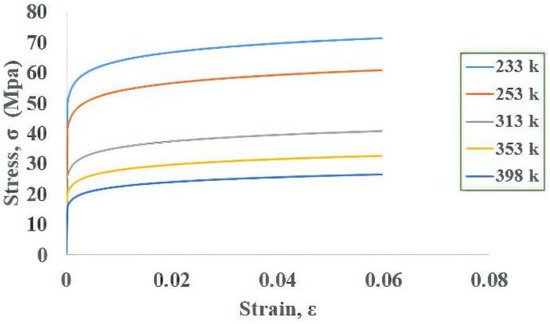
In the simulation process, the solder material was a nonlinear plastic material. Therefore, PLANE182, which has good convergence characteristics and can deal with large deformations, was used as the solder ball element. Figure 23 shows the stress–strain curve for an Sn–Ag–Cu (SAC)305 solder joint. The stress–strain curve ^[22][56], obtained by tensile testing and the Chabochee kinematic hardening model, was used to describe the tensile curves at different temperatures. Once the model is built, boundary conditions and external thermal loading are required for the WLP simulation.

Figure 23.

Stress–strain curve for SAC solder.

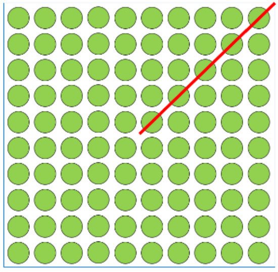
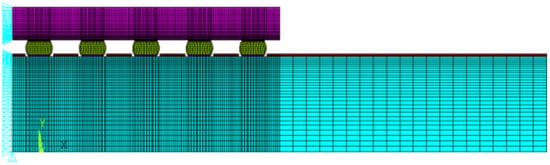
Electronics packaging geometry is usually symmetrical; therefore, in this study, half of the 2D structure was modeled along the diagonal, as shown in Figure 34. The X-direction displacement on each node was fixed to zero owing to the Y-symmetry. To prevent rigid body motion, the node at the lowest point of the neutral axis, which is at the printed circuit board (PCB), has all degrees of freedom fixed. The complete finite element model and the boundary conditions are shown in Figure 45. The thermal loading condition used in this research was JEDEC JESD22-A104D condition G ^[23][57], and the temperature range was −40 °C to 125 °C. The ramp rate was fixed at 16.5 °C/min and the dwell time was 10 min. In a qualified design, its mean-cycle-to-failure (MTTF) should pass 1000 thermal cycles. After the simulation process is completed, the incremental equivalent plastic strain in the critical zone is substituted into the strain-based Coffin–Manson model ^[24][58] for reliable life cycle prediction. For a fixed temperature ramp rate, this method is as accurate as the energy-based empirical equation ^[25][26][59,60] but with much less CPU time.

Figure 34.

Symmetrical solder ball geometry.

Figure 45.

FEM model boundary condition.

The empirical formula for Coffin–Manson equivalent plastic strain model is shown in Equation (1):

Table 15 presents the predicted reliability life cycles of the WLP structure. The results show that the difference between the FEM-predicted life cycle and experiment result is within a small range. Therefore, experiments can be replaced by this validated FEM simulation to minimize the cost and time. Compared with the experiment approach, this validated FEM simulation procedure can provide large amounts of data within much less time and can be effectively used to generate a database for AI training.

Table 15.

WLP finite element results for five test vehicles.

Test Vehicle	Experimental Reliability (Cycles)	Simulation Reliability (Cycles)	Difference

TV1	318	313	−5
TV2	1013	982	−31
TV3	587	587	0
TV4	876	804	72
TV5	904	885	19

3. Machine Learning

3.1. Establishment of Dataset

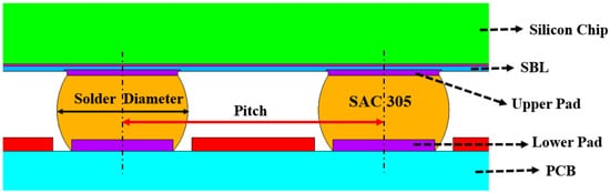
The WLP structure consists of several components, including the solder mask, solder ball, I/O pad, stress buffer layer, and silicon chip, etc. (Figure 56). For illustration purposes, the four most influential parameters, namely silicon chip thickness, stress buffer layer thickness, upper pad diameters, and lower pad diameters, were selected to build the AI model and predict the reliability life cycles of new WLP structures. These four design parameters were used to generate both training and testing datasets for AI machine learning algorithms. Table 26 and Table 37 show the generated training dataset obtained through FEM simulation.

Figure 56.

WLP geometry structure.

3.2. ANN Model

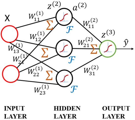
The ANN model is based on the concept of the brain’s self-learning ability, mimicking the human nervous system to process information. It is a multilayer neural network, as shown in Figure 67. The model consists of three layers: the input layer, where the data are provided; the hidden layer, where the input data are calculated; and the output layer, where the results are displayed ^[27][63]. As the numbers of neurons and hidden layers are increased, the ability to handle nonlinearity improves. However, these conditions may result in high computational complexity, overfitting, and poor predictive performance.

Figure 67.

Schematic diagram of artificial neural network.

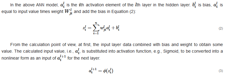
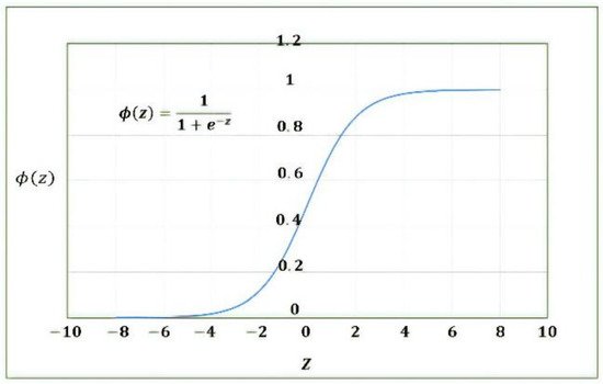
where the activation function is shown in Figure 78.

Figure 78.

Sigmoid activation function.

3.3. RNN Model

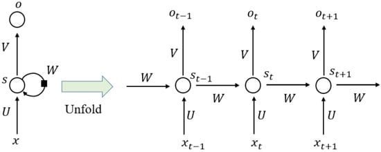
RNN is a type of neural network that can model “time-like”-series data, and it commonly adopts a nonlinear structure in deep learning. RNN ^[28][29][64,65] works on the principle that the output of a particular layer is fed back to the input layer to realize a time-dependent neural network and a dynamic model. Consequently, an ANN with nodes connected in a ring shape is obtained, as shown in the left half of Figure Figure 89. 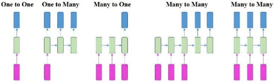The ring-shaped neural network is expanded along the “time” axis, as shown in the right half of Figure 8Figure 9, where the “time” step t and the hidden state st can be expressed as a function of the output from the previous (st−1) “time” steps and previous layers (xt). U, V, and W denote the shared weights in RNN models during different “time” steps. Generally, the RNN series model can be divided into four types according to the number of inputs and outputs in given “time” steps; that is, one to one (O to O), one to many (O to M), many to one (M to O), and many to many (M to M). To synchronize the input features with the output results, RNN models can be subdivided into different series models, as shown in Figure 9Figure 10 ^[30][66].

Figure 89.

Schematic structure of recurrent neural network.

Figure 910.

Different series model for RNN.

3.4. SVR Model

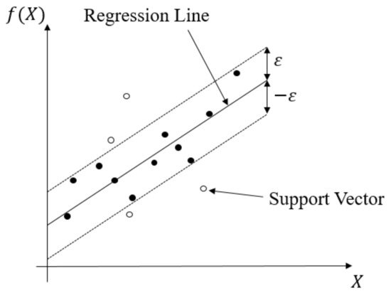
This regression method evolved from the support vector machine algorithm. It transforms data to high-dimensional feature space and adapts the ε-insensitive loss function (Equation (4)) to perform the linear regression in feature space (Equation (5)). In this regression method, the norm value of w is also minimized to avoid the overfitting problem. In other words, f(X,w), which is the function of the SVR model, will be as flat as possible. The SVR concept is illustrated in Figure 10Figure 11. The data points outside the ε-insensitive zone are called support vectors, and two slack variables, ξi and ξ∗i, are used to record the loss of each support vector. Thus, the whole SVR problem can be seen as an optimization problem (Equation (6)).

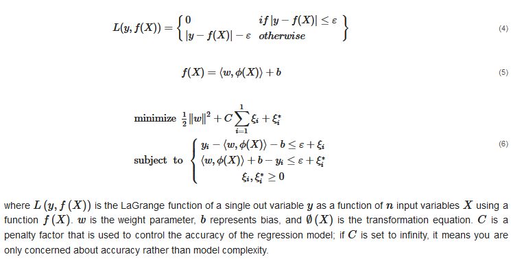
Figure 110.

Schematic diagram of SVR.

In order to solve the optimization problem, the regression model is built as shown in Equation (7), where b is the bias of the SVR model.

In Equation (7), the term K(X,Xi) is known as the kernel function, and Xi is the training sample, with X as an input variable. This kernel function should be chosen as a dot product in the high-dimensional feature space [67]. There are numerous types of kernel functions. The commonly used kernel functions for SVR are the linear kernel, polynomial kernel, radial basis function (RBF) kernel, and sigmoid kernel.

All of the kernel functions satisfy Mercer’s condition; however, the regression results of the kernels vary. Therefore, it is essential to choose the best kernel function for the SVR algorithm to obtain optimal performance.

3.5. KRR Model

KRR combines ridge regression with the kernel “trick”. This model can learn a linear function in the space induced by the respective kernel and the dataset. Nonlinear functions in the original space can be used by the nonlinear kernels. The KRR algorithm also analyzes several kernels such as the RBF kernel, sigmoid kernel, and polynomial kernel to find the suitable kernel function for the WLP nonlinear dataset.

The KRR is possibly the most elementary algorithm that can be kernelized to ridge regression ^[31][68]. The classic method is used to minimize the quadratic cost, as shown in Equation (8). However, for the nonlinear dataset, the lower-dimensional feature space replaces the higher-dimensional feature space; that is, Xi→Φ(Xi). To convert lower-dimensional space to higher-dimensional space, the predictive model undergoes overfitting. Hence, to avoid overfitting, this function requires regularization.

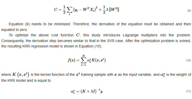
Hence, Equation (11) is very simple and more flexible due to introducing kernel function K, $λ$ is the regularize factor with the identity matrix I, and $y$ is the response variable. This model can also avoid both model complexity and computational time.

3.6. KNN Model

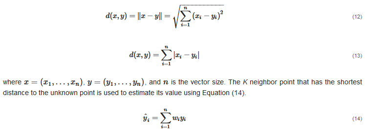
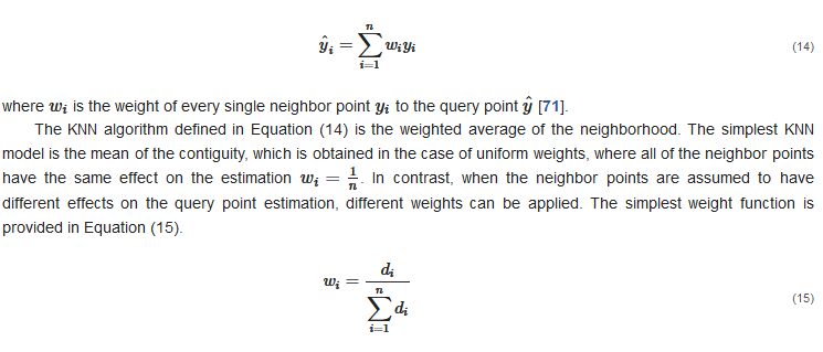
The KNN model is a statistical tool for estimating the value of an unknown point based on its nearest neighbors [69]. The nearest neighbors are usually calculated as the points with the shortest distance to the unknown point [70]. Several techniques are used to measure the distance between the neighbors. Two simple techniques are used in this study: the Euclidean distance function d(x,y), provided in Equation (12), and the Manhattan distance function d(x,y), provided in Equation (13).

3.7. The RF Regression Model

RF is a collection of decision trees. These tree models usually consist of fully grown and unpruned CARTs.

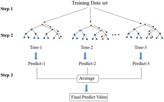
The structure of the RF regression model is shown in Figure 101. This algorithm creates an RF by combining several decision trees built from the training dataset. The CART tree selects one feature from all of the input features as the segmentation condition according to the minimum mean square error method.

The RF algorithm procedure comprises three steps. In step 1, the bagging method is used to create a subset that accounts for approximately 2/3 of the total data volume. In step 2, if the data value is greater than the selected feature value, the data points are separated to the right from the parent node, otherwise to the left of the parent node (Figure 112). Afterward, a set of trained decision trees is created. In step 3, the RF calculates the average value of all decision tree results to obtain the final predicted value.

Figure 112.

Schematic diagram of random forest structure.

3.8. Training Methodology

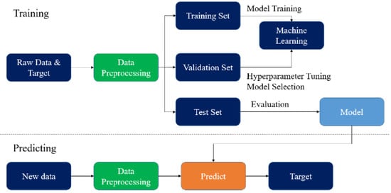
To obtain the best performance and avoid overfitting of the final trained regression model, several techniques, including data preprocessing (for standardization), cross-validation (for parameter selection), and grid search (for hyperparameter determination), were applied during training. The AI regression model was estimated using the method in the flowchart given in Figure 123.

Figure 123.

Methodology flow chart.

3.8.1. Data Preprocessing

The dataset values are not in a uniform range. Hence, before the machine learning model is developed, the data need to be preprocessed to standardize all of the input and output datasets and improve the modeling performance. Several data preprocessing methods, including min–max scaling, robust scaling, max absolute scaling, and standard scaling, were used in this study. Hence, of all preprocessing methods, we need to select the one method that provides the most accurately predicted output from the input dataset.

3.8.2. Cross-Validation

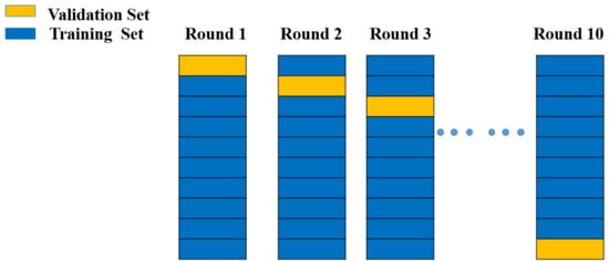
Cross-validation is the most frequently used parameter selection method. The basic idea of cross-validation is that not all of the dataset is used for training; a part of it (which does not participate in training) is used to test the parameters generated by the training set. The training data are trained with different model parameters and verified by the validation set to determine the most appropriate model parameters. Cross-validation methods can be divided into three categories: the hold-out method, k-fold method, and leave-one-out method. Owing to the huge calculation burdens of the hold-out method and the leave-one-out method, the k-fold method was chosen for this study (Figure 134). After the choice of data preprocessing method was confirmed, cross-validation was performed to avoid overfitting of the machine learning model, as shown in Figure 134. The dataset was divided into 10 parts, and each part acted as either a validation or training set in different training steps. The validation sets were also used to predict the training results.

Figure 134.

Cross-validation model diagram from Round 1 to Round 10.

3.8.3. Grid Search Technique

Grid search is a large-scale method for finding the best hyperparameter to build the training model. In order to determine the best parameter, the search range value needs to be set by the model builder. Although the method is simple and easy to perform, it is time-consuming. Therefore, to reduce the computation time, this work adopted the grid search technique to find the best hyperparameter as compared to manually searching the hypermeter, and eventually, the training model was fixed with the above hyperparameters to run the best AI model.