1. Introduction

The 1921 Nobel Prize in Physics was awarded to Albert Einstein “for his services to Theoretical Physics, and especially for his discovery of the law of the photoelectric effect” [1]. This exciting discovery further inspired humanity’s futuristic dream to harness the sun for free energy. While indeed free and, in some parts of the world, abundant, solar energy is still challenging to capture, store and distribute to users on an economical basis. The primary disadvantages of solar energy generation systems are their intermittent nature, the limited conversion efficiency of commercially available photovoltaic (PV) cells, and the high capital investment. The cost of the solar generation system can be reduced by improving the photovoltaic conversion efficiency so that smaller and cheaper systems can be used. Less hardware, installation, labor, and real estate costs can improve the Total Life Cycle Cost of solar energy [2] and, consequently, increase the penetration of solar energy generation systems into the global energy market.

The small physical dimensions of a PV cell allow limited amount of solar irradiation to be captured, providing only a minute amount of electrical power. To generate a practically usable amount of energy, a large number of PV cells have to be stacked together to form an array, also referred to as a PV panel or single PV module. Commercially available PV modules are field-installable units, typically 1–3 sq. m in size, which can generate about 150–300 W each. Grid-connected PV generating systems are designed to supply much higher power and require a considerable amount of PV modules to be assembled into a larger PV array [3]. Thus, the PV array is, in fact, an array of arrays composed of a huge number of basic PV cells and has complex wiring. The optimal utilization of such a large ensemble of PV cells is a rather intricate task.

The primary challenge is posed by the inherent non-linearity of the PV cell, that has a bell shape power-voltage curve with a unique maximum power point (MPP). The MPP is located at the knee of the voltage-current characteristics, where the abrupt slope change manifests the transition from current source behavior towards the voltage source region. Yet, in case of shading or malfunction, the P–V curve may comprise several distinct MPPs. Therefore, to extract the maximum available DC power out of the PV array, an electronic dynamic Maximum Power Point Tracker (MPPT) [4] and a proper power converter/inverter set are required to generate AC at utility compatible voltage level and connect to the grid.

The wiring of the PV array, the power processing architecture and the MPPT algorithm have a significant effect on how the mismatch and shading affect the power yield of the PV system ^[5][6]. Over the years, researchers have extensively experimented with various PV architectures to maximize the energy yield of PV sources and make the system fault-tolerant, forbearing mismatch, and shading problems, while keeping the solution economically viable. To date, a formidable body of theoretical knowledge supported by extensive practical experience has been accumulated ^[6][5].

2. Static PV Arrays

To help limit the mismatch and shading effects, the wiring pattern of the PV array has to be considered to identify architecture with sufficient redundancy. Several possible PV arrays’ interconnection schemes were reported early in the literature ^[7][8][7,8]. These include the Series (S); the Parallel (P); the Series–Parallel (SP); the Series–Parallel–Series (SPS); the Total-Cross-Tied (TCT); the Bridge-Linked (BL); and the Honey-Comb (HC) arrays, illustrated in Figure 1 a–g, respectively. A simple S array can attain high output voltage at low output current while the P array can provide the highest output current, but only at the low output voltage. The S array is also referred to as the string, whereas the P array is the tier. Both S and P arrays have the simplest wiring. The SP array can output both a high voltage and high current, yet it has simple wiring. The SPS array is formed by connecting several short SP sub-arrays in series.

Figure 1. Common configurations of PV arrays: Series (a); Parallel (b); Series–Parallel (c); Series–Parallel–Series (d); Total-Cross-Tied (e); Bridge-Linked (f); Honey-Comb (g).

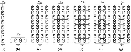
The TCT array is a string of PV tiers and has a simple setup but also the longest wiring. The BL array has its modules interconnected in bridge rectifier fashion and has a rather complex interconnection. The “honeycomb” pattern of the HC array can be revealed when Figure 1 g is “stretched” horizontally. The HC array has the most complex wiring, which is less of a problem for PV modules manufacturers, but can be demanding for constructing large field installations. In the ideal case, SP, SPS, TCT, BL, and HC arrays can all provide the same high voltage and current; however, the merits of these arrays are in their ability to cope with shading conditions.

The shape of the array’s V –I curve changes when shadows are cast. While P arrays tend to maintain an easier-to-track single MPP, the composite V –I curve of the S array may include several local maxima points ^[9][10]. Both occur due to mismatch losses, and losses due to failure in tracking the global MPP the long S and SP arrays are more prone to loss of power than the short SP or short SPS arrays. Short strings controlled individually seem to deliver the most reliable power production ^[10][13]. Therefore, increasing tolerance to shading conditions and the maximization of the energy yield of PV arrays necessitates a minimization of string length. This is especially important in an urban environment, such as roof-top and building-integrated PV systems.

Further comparison of the three popular high-voltage array architectures reveals that the BL array has the best performance under shading conditions, whereas the TCT array was found second best, and SPS is the least tolerant to shading effects ^[11][14].

3. Variable Structure Arrays

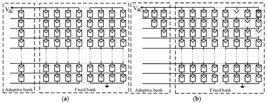
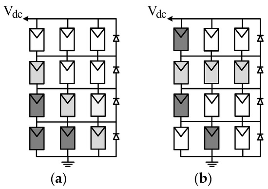
In normal conditions, the modules of the reconfigurable array are distributed equally in parallel to the tires of the main TCT array—see Figure 26 a. To equalize the energy production of the array under shading conditions, one or more PV modules from the adaptive bank are removed from the strongest tire and relocated in parallel to the weakest tire. The sorting continues until all the modules of the adaptive bank are redistributed, as in Figure 26 b. Partial shading of a particular tire manifests itself by slightly decreased voltage. Therefore, electrically, the objective of the controller is to minimize the differences in voltage measured across the tires. DPVA requires additional hardware and complex sorting and control algorithms to be applied.

Figure 26. Dynamic PV Array: during uniform insolation conditions (a); reconfigured to compensate for partial shading (b) ^[12][21].

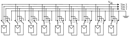
To implement a reconfigurable array having a hard-wired fixed part of TCT array and an adaptive one of independent solar cells, both parts were linked through a controllable matrix of switches ^[13][22]. The matrix, see Figure 37 , was controlled in real time to connect the cells of the adaptive array in parallel with shaded rows of the fixed one and optimize the output power.

Figure 37. Switching Matrix for a reconfigurable 3 × 3 TCT array (normal configuration) ^[13][22].

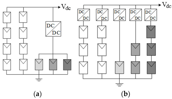
The principle of the optimized string-configured DPVA (OS-DPVA) ^[14][24] is configuring the PV modules into several strings with similar power levels. Each string connects to the dc bus through an MPPT dc–dc converter, as shown in Figure 48 b. The number of strings is determined according to the number of available dc–dc converters. Under these constraints, the controller evaluates the most productive array arrangement for the given environmental conditions. As the string length is unpredictable, the input voltage to the dc–dc converter may vary widely.

Figure 48. String-Configured Dynamic PV Array (a) ^[15][23]; the Optimized String-Configured Dynamic PV Array (b) ^[14][24].

To optimize the productivity of the TCT array, the authors of ^[13][22] suggested reconfiguring the array to equalize tire currents. Since the photocurrent is directly proportional to the irradiation, the method also aims to do this; therefore, it also is referred to as the Irradiance Equalization (IEq). The approach is implemented by relocating modules from the best-performing tire to the weakest one until the IEq is achieved, as shown in Figure 59 . The optimum irradiation of a tire can be found by averaging the total irradiation captured by the array per number of tires.

Figure 59. Illustration of the reconfiguration strategy: initial (a); irradiance equalized (b) ^[13][22].

4. Power Processing Architectures for PV Arrays

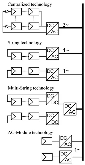
Another key component of any solar energy generation plant is the electronic power inverter. The inverter’s task is interfacing the solar energy to the grid. This involves maximum power point tracking (MPPT) function to maximize the captured energy, converting the dc voltage obtained from the PV array into AC, and injecting it to the grid in compliance with the high-power quality standards, i.e., at high power factor and minimum harmonic distortion. The inverter’s architecture is concerned with the implementation of a certain operational strategy of a PV array that can maximize its energy output. Four major PV inverter concepts, shown in Figure 611 , are the centralized inverter, the string inverter, the multi-string inverter, and the micro-inverter ^[16][25]. The centralized inverter system is designed to connect a large SP array to the grid. SP array can provide sufficiently high voltage and high power, that justifies a three-phase grid connection with the additional advantage of reduced dc–ac power decoupling requirements.

Figure 611. Commonly used PV inverter types ^[16][25].

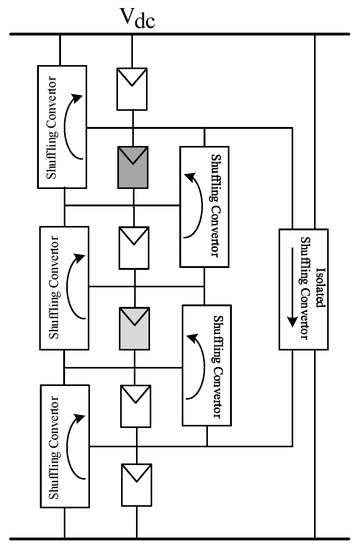
The power loss of a PV string to partial shading can be minimized by applying low-power dc–dc converters, which can “shuffle” power around a problematic module. The converters are wired in overlapping arrangement to shuffle power one level up, as illustrated in Figure 718 ^[17][38]. The shuffling converter has to process only the small difference between the powers generated by the adjacent modules. Therefore, while the shuffling converters can significantly increase the power generation under shading conditions, the converter losses have only a marginal effect on the overall system efficiency. However, in the worst case of mismatch, when the PV module has lost most of its generation capacity, the power shuffled by a converter equals that of a PV module so the converter must be rated accordingly. Since the system in Figure 718 is composed of unidirectional converters, it also requires an isolated converter unit to shuffle power from the top to the bottom of the string. The top-to-bottom shuffling unit can be spared when using bidirectional converters such as non-isolated Cuk or buck-boost/flyback converters ^[18][39].

Figure 718. PV string with shuffling equalization scheme.

Application of a dedicated converter per each PV module is referred to as Module-Integrated Converter (MIC). MIC is individually controlled by the MPPT controller to extract the optimal amount of available power from each PV module and help to resolve mismatch and shading problems. MICs that are employed as dc–dc converters are referred to as dc optimizers, whereas MICs with a dc–ac inversion capability can be connected directly to the grid and are commonly referred to as micro-inverters. Compared to equalizers, which process only part of the power needed to balance the PV array, MICs process the full power of the array and are at disadvantage. For these reasons, MICs have to exhibit the highest efficiency, whereas the requirements towards the equalizer’s performance are significantly relaxed.

5. Sub-Module Power Processing Architectures

PV modules are pre-wired, field-installable units fabricated in a variety of sizes and rated voltage and power output. To date, the 36- and 72-cell PV modules are the industry standards for large power production ^[19][20][21][61,62,63]. Most commercially available PV modules are configured as a short string of a few, usually three, sub-strings, each having a bypass diode across. Each sub-string is configured as an SP array of macro-PV cells. The incentive to the investigation of sub-module architectures remains increasing the energy yield of a single PV module by reducing the limitations set by mismatch and partial shading. Various approaches developed for string and module levels can also be applied to maximize the power output from each sub-string within the partially shaded PV module. This calls for application of power optimizers, equalizers and MPPT techniques similarly to the described above.