Computer modeling of the electrophysiology of the heart has undergone significant progress. A healthy heart can be modeled starting from the ion channels via the spread of a depolarization wave on a realistic geometry of the human heart up to the potentials on the body surface and the ECG.
1. Introduction
This article reviews research aimed at building a bridge between computerized modeling of the electrophysiology of the human heart and the analysis of the electrocardiogram (ECG). Potential applications of computer modeling for better interpretation of the ECG are demonstrated and an outlook for further research is given.
The research field of computerized modeling of the electrophysiology of the heart has reached a mature state. The healthy heart can be replicated in a computer model with various degrees of detail, starting with the ion channels and ending with the spread of a depolarization wave through the atria and the ventricles. Several diseases have been the focus of this research but many open questions remain: modeling can only be as good as our basic understanding of the pathologies of the heart.
On the other hand, after more than 100 years of ECG interpretation, the clinical knowledge about ECG and what it can tell us about cardiac diseases has reached an expert level. Most often, this knowledge is based on personal experience or empirical studies and only coarse attempts are made to relate a decisive feature in the ECG to its pathological origin inside the heart. The classical heart vector is a valuable tool for understanding the general shape of the ECG, but it is not good enough to follow details of the spatial spread of de- and repolarization.
It is astounding that the number of articles where modeling of the heart is extended to the calculation of the ECG and where this is used for better ECG interpretation is limited. Table 1 shows the result of a literature survey.
Table 1. Literature survey of research about modeling of the heart together with the corresponding ECG.
| Topic |
Modeling Challenge |
References |
| healthy heart—QRS |
modeling the Purkinje tree |
[1][2][3][4][5]9] | [1,2,3,4 | [6][7][ | ,5 | 8 | ,6 | ] | ,7,8 | [ | ,9] |
| healthy heart—T-wave |
modeling heterogeneity of repolarization |
[10][11][12] | [10 | [ | ,11 | 13 | ,12 | ] | ,13] |
| healthy heart—P-wave |
modeling sinus node excitation and pathways from right to left atrium, anatomical variability |
[14][15][16][17][18][19[22] | [14,15 | ][ | ,16 | 20][ | ,17 | 21 | ,18 | ] | ,19,20,21,22] |
| ischemia and infarction |
modeling the effect of hyperkalemia, acidosis, hypoxia and cell-to-cell uncoupling |
[23][24][25][26][27][28][29][30] | [23,24,25,26,27,28,29,30] |
| ventricular ectopic beats |
localization with 12-lead ECG |
[31][32][33][34] | [31,32,33,34] |
| ventricular tachycardia |
localization of exit points with 12-lead ECG |
[29][35] | [29,35] |
| cardiomyopathy |
modeling typical changes of QRS- and T-wave |
[36] |
| bundle branch blocks LBBB and RBBB |
modeling asynchrony |
[37][38][39][40] | [37,38,39,40] |
| atrial ectopic beats |
localization with 12-lead ECG |
[32][33][34] | [32,33,34] |
| atrial tachycardia, flutter |
modeling all types of flutter |
[20][41][42][43][44][45][46] | [20,41,42,43,44,45,46] |
| atrial fibrillation and fibrosis |
modeling fibrosis and its distribution |
[47][48][49][50][51] | [47,48,49,50,51] |
| genetic diseases |
modeling LQT, SQT, Brugada |
[52][53][54] | [52,53,54] |
| imbalance of electrolytes |
hyper- and hypokalemia and hyper- and hypocalcemia |
[13][55][56][57][58][59][60] | [13,55,56,57,58,59,60] |
| drug-induced changes |
effect of various channel blockers |
[61][62][63] | [61,62,63] |
Methods for calculation of the ECG (and the body surface potential map, BSPM) from the source distribution in the heart have been described in several articles. The main differences between the approaches are (a) the cellular models and their parameters, (b) the method to calculate the spread of depolarization (bidomain, monodomain, eikonal, reaction eikonal) and (c) the method of forward calculation (finite difference, finite element, boundary element methods; homogeneous torso versus different organs considered). The forward problem is obviously related to the inverse problem of ECG as used in ECG imaging (ECGi). Thus, all articles dealing with fast and realistic methods of calculating the lead field matrix that maps the sources in the heart to the body surface ECG are related to the topic of this article but are not discussed in detail.
Published in 2004, the software package ECGSim allows for a fast and easy relation of source patterns on the heart to the corresponding 12-lead ECG. The user can modify local activation times, repolarization times and the slope of the transmembrane voltage
[64]. Thus, these source distributions can be realistic or not—no model of excitation spread is running in the background. Meanwhile, advanced software packages to simulate the electrophysiology of the heart are available: openCARP
[65][66][65,66], acCELLerate
[67], FEniCS
[68], Chaste
[69], propag-5
[70], and LifeV
[71]. They all have been verified in an N-version benchmark activity initiated by Niederer
[72].
The literature survey yielded several articles that do not focus on a specific disease but rather deal with the general concept of calculating the ECG from computer models of the heart. Lyon et al. gave an outline of a computational pipeline, listed examples of modeling diseases together with the ECG and showed up several applications of modeling in ECG interpretation
[73]. Potse suggested a fast method for realistic ECG simulation without oversimplifying the torso model by using a lead-field approach
[74]. Building upon this approach, Pezzuto et al. found an even faster method that allows for implementation on a general-purpose graphic processing unit (GPGPU)
[75]. Keller et al. investigated the influence of tissue conductivities on the resulting ECG
[76]. Schuler et al.
[77] found a way to downsample the fine grid necessary for calculating the spread of depolarization for the forward calculation of the ECG—further reducing calculation time. Neic et al. developed a reaction eikonal algorithm that simulates the spread of depolarization very fast and still delivers realistic ECGs
[78].
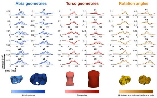
Calculation times for computing the spread of depolarization and repolarization, the lead field matrix and the body surface potentials including the ECG strongly depend on the methods employed: highly detailed cell models versus simplified phenomenological models, high versus low spatial resolutions, etc. They can range from one day down to one second. As an example, the calculation times of the P-waves shown in Figure 1 were 27 h for the full bidomain model and the Courtemanche cell model, 1 h and 24 min for a pseudo-bidomain model and 40 min for a monodomain simulation (heart mesh with 4.7 million elements and 920 k nodes, desktop computer with 12 cores at 1.4 GHz). Fast calculation times are important for the researcher aiming at the identification of new features in the ECG, for creating a training dataset for machine learning and for personalization of a heart model. They are not relevant any more if, for example, a machine learning algorithm is finally used in clinics.
Figure 1. Simulated P-waves of the 12-lead ECG with various atrial shapes, several orientations of the atria inside the torso and a variety of body shapes. The colors represent the total atrial volume in blue, the torso size in red and the orientation angle around the medial-lateral axis in orange
[50].
2. Modeling the ECG of a Healthy Heart
2.1. The QRS Complex and the Purkinje Tree
The morphology of the QRS complex is strongly determined by the topology of the His-Purkinje system in the ventricular subendocardial layer
[2]. An earlier approach to fit a Punkinje network model to a measured ECG was published by Keller et al. in 2009
[1]. In total, 744 Purkinje muscle junctions were distributed across the ventricular endocardial surface following specific rules. Other publications followed this scheme and implemented “root points” coupled to thin endocardial layers with very fast conduction
[3]. Automatic and reproducible manipulation of root node locations is facilitated by chamber-specific coordinate systems
[79][80][81][79,80,81]. Mincholé et al. investigated the impact of anatomical variability on simulated QRS complexes
[6]. They found that QRS duration is mainly determined by myocardial volume and not affected by the position of the heart in the torso. The latter influences QRS morphology in the precordial leads, whereas ventricular anatomy dominates in the limb leads. Cranford et al. carried out a sensitivity study: they implemented 1 to 4 “seed stimuli” and up to 384 “regional stimuli” and observed the changes in the QRS complex while changing the number and topology of excitation sites
[5]. The topology of four seed stimuli at adapted positions was more relevant than a large number of regional stimuli. Pezzuto et al. were able to reproduce the QRS complex of 11 patients using up to 11 of the earliest activation sites on the endocardium and adapted the conduction velocity in the ventricles and in a fast endocardial layer
[7]. Gillette et al. proposed a comprehensive workflow to optimize the positioning of five root disks, timing, and endocardial conduction velocities (10 parameters) to reproduce the QRS complex with a personalized model
[8].
The healthy QRS complex can be reproduced faithfully, meaning that adapted heart models show an ECG with high correlation to measured ECGs. This does not prove that the modeled spread of depolarization is the one present in the patient, but it is good to see that there are no inconsistencies. Some relevant questions are: Which parameters in the model are responsible for the natural variability of QRS complexes—both inter- and intra-patient wise
[4][6][4,6] (see also Section 2.5)? Is the heart axis that is visible in the ECG mainly determined by the geometrical axis of the heart or by the properties of the His-Purkinje system? Which simplifications of the thorax model are acceptable and where do we need detailed models?
2.2. The T-Wave and the Repolarization
Modeling the T-wave is a challenging task. If all myocytes in the ventricles would follow the same action potential, the T-wave would have the opposite sign as the R-peak. Heterogeneity is a necessary condition for concordant T-waves. Keller et al. investigated various schemes of heterogeneity of the IKs
repolarization current (transmural, apico-basal, left–right) and found that both transmural and apico-basal gradients can lead to realistic T-waves, whereas a pure left–right heterogeneity creates a notch in the T-wave [11]. Even though the focus of an article of Bukhari et al. was on the changes in the T-wave during dialysis (see Section 3.9), this article also reported on the heterogeneity that is needed to obtain a realistic T-wave in healthy hearts. They assume a solely transmural dispersion of ion channel conductivities [13]. Xue et al. analyzed how transmural and apico-basal heterogeneities change the morphology of the T-wave. They concluded that mainly apico-basal gradients contribute to a positive T-Wave [10]. The mocludeled heterogeneity scenarios are informed by experimental cellular data [82]. However, ties of the available data do nfot allow us to draw definite conclusions and different heterogeneity patternsllowing ion channels: canIKs, leadIKr, to the similar T-wave morphologies.Ito
. They concluded that mainly apico-basal gradients contribute to a positive T-W
ave [10]. Th
e modeled heterogenei
le ty scenarios are informed by experimental cellular data [82]. However, the available data do not allow us to draw definite con
clusions and different
ractio heterogeneity patterns can lead to the similar T-wave morphologies.
While con
traction of the heart happens only after the P-wave and the early QRS complex, it can influence the source distribution during the repolarization. How the contraction of the heart affects the morphology of the simulated T-wave was investigated by Moss et al. They observed an 8% increase in amplitude and a shift of the T-wave peak by 7 ms
[12].
2.3. The P-Wave
A review about computerized modeling of the atria including the corresponding ECG was given by Doessel et al. in 2012
[15]. Krueger et al. were the first to set up an atrial model that included realistic fiber orientation
[14][83][14,83]. They also investigated the influence of atrial heterogeneities on the morphology of the P-wave, created personalized models and compared the ECGs of several patients
[16].
The contribution of the left and right atria to the P-wave was analyzed by Loewe et al.
[17] and Jacquemet et al.
[18]. Even in the last third of the P-wave, one-third of the signal stems from the right atrium
[17]. Potse et al. discovered that a jigging morphology of the P-wave, which was observed in computer simulations, was not an artefact but could be observed in a similar way in healthy volunteers when carefully preventing smoothing through filtering or averaging
[19]. Loewe et al. investigated the influence of the earliest site of activation in the right atrium (i.e., the sinus node exit site) on the morphology of the P-wave
[20] and could demonstrate that small shifts in the earliest excitation site and its proximity to the inter-atrial connections can significantly change the terminal phase of the P-wave. Andlauer et al. dissected the differential effects of atrial dilation and hypertrophy on the morphology of the P-wave
[21] and showed that left atrial dilation did not influence P-wave duration significantly, but instead had a strong effect on P-wave amplitude and thus P-wave Terminal Force in lead V1 (PTF-V1).
A literature survey of simulations of the P-wave and in particular of the P-wave in patients suffering from paroxysmal atrial fibrillation (AFib) was published by Filos et al.
[43]. All the effects described in the literature that have an influence on the morphology of the P-wave of AFib patients are outlined. Despite the very large number of articles, we conclude that there is still a way to go before these results can be routinely used in clinical practice.
Nagel et al. analyzed the inter- and intra-patient variability of the P-wave in the Physionet ECG database, aiming at the optimization of a simulated database of P-waves
[84][84] (see also Section 2.5).
Figure 1 shows several examples of P-waves with various atrial shapes, several orientations of the atria inside the torso and a variety of body shapes.
2.4. Modeling Rhythmic Features and Heart Rate Variability
Modeling of a heart beat most often starts with a stimulation either from an area around the sinus node (atria) or from the model of the Purkinje tr
ee
e (ventricles, see Section 2.1). Modeling of the sinus node is an interesting research topic that goes beyond the scope of this article.
The ECG fluctuates from beat to beat even in the healthy state. Both the RR interval and also the morphology of the P-, QRS- and T-wave are not completely periodic. The fluctuations of the RR interval are well known and analyzed by means of heart rate variability (HRV), as reviewed by Rajendra et al.
[85]. HRV is high in normal hearts and low when there is a cardiac problem. The variation in the beat-to-beat RR interval is usually studied in both the time domain and frequency domain. Not many clinicians make use of this measure in daily clinical practice. On the modeling side, only few articles describe simulations of beta-adrenergic and vagal tones on the sinus node
[86]. It seems as if there is still a “missing link” between computerized modeling of the heart and HRV interpretation
[87].
2.5. Modeling Inter- and Intra-Patient Variability
The variety of ECG morphologies observed in a cohort of healthy humans is large. This can be explained by different geometries of the heart
[88] , different rotation inside the thorax
[6], and different shapes of the torso. Moreover, differences in electrophysiology also contribute to the variability (see, for example, the discussion about the QRS morphology and the Purkinje tree in
Section 2.1).
As already mentioned in
Section 2.3, Nagel et al. investigated the inter- and intra-patient variability of the P-wave
[84]. The beat-to-beat variability of the P-wave in case of atrial fibrillation was investigated by Pezzuto et al.
[42]. Already small variations (1 to 5 mm) in the location of the earliest activation site lead to changes in the morphology of the P-wave. This effect was significantly enhanced if slow conducting regions were near the earliest activation site.
3. Modeling Diseases and the Corresponding ECG
3.1. Ischemia and Infarction
Loewe at al. gave an outline of how computer modeling can support comprehension of cardiac ischemia and discussed the link to the corresponding ECG
[28].
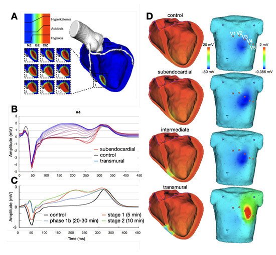
Figure 2 shows several examples of ischemic regions together with the corresponding ECG. The parameters of the ten Tusscher–Panfilov cell model which reflect the degree and temporal stage of the occlusion were summarized by Wilhelms et al.
[25]. They considered the cellular effects due to hyperkalemia, acidosis and hypoxia as well as due to cellular uncoupling. After clarifying the origin of ST-segment elevation (and depression), they also demonstrated how several ischemic scenarios will not show any ST-segment change
[26]. Thus, they were able to explain the large group of non-ST-segment elevation myocardial infarctions (NSTEMI). Potyagaylo et al. showed that these scenarios are not only electrically but also magnetically “silent”
[89]. Loewe at al.—using computer modeling—investigated whether additional electrodes, optimized electrode placement or improved analysis of the ST segment could lead to better diagnosis of patients with acute ischemia. They suggest the deviation from baseline at the K-point as being superior to J-point analysis
[27].
Figure 2. Examples of ischemic regions with varying transmural extent due to occlusion of the left anterior descending coronary artery and the related levels of hyperkalemia, acidosis, and hypoxia (
A). ECG lead V4 for ischemia of varying transmural extent in temporal stage 2 (
B) and varying duration of a transmural ischemia (
C). Ventricular transmembrane voltage and body surface potential distribution during the action potential plateau (t = 200 ms) for ischemia of varying transmural extent in stage 2 (
D). The QRS complex was not optimized in this study. (Images reproduced with permission from
[28].)
Ledezma et al. created populations of control and ischemic cell strands and observed the corresponding pseudo-ECGs (which is the voltage between two virtual electrodes at or near to the ends of a tissue strand immersed in an infinite homogeneous volume conductor). Based on these data, they trained an artificial neural network that was able to determine severity (mild or severe) and size of the ischemic region from the pseudo-ECG
[30].
All these articles deal with ischemia and “fresh” infarctions (not older than a couple of hours). The modeling of “old” infarction scars seems to be straightforward: the scar areas cannot depolarize, they should be “switched off” during modeling. Basically. the QRS complex will change. In particular, small bridges of viable tissue within a scar area are of interest since they are likely to lead to ventricular tachycardia (VT). Lopez-Perez et al. were able to set up a personalized model of a patient with an old infarction with strong emphasis on modeling border zones. They were able to reproduce the 12-lead ECG of a patient with a history of infarction both in sinus rhythm and during VT
[29](see Section 3.3) [29].
Electrocardiographic imaging of myocardial infarction was the subject of the Challenge of the Computing in Cardiology conference in 2007. BSPMs of patients were provided for the participants. Ghasemi et al. were very successful in finding the location and extent of the infarction using only the heart vector and a very simplified model of the distribution of depolarization during systole
[90]. Farina et al. employed a model-based approach to solve the task
[23] and also reached very good results; however, based on the full BSPM. Jiang et al. investigated the best electrode arrangements to localize an infarcted area in the heart
[24]. A dense set of electrodes including and extending the precordial leads was essential. Optimal results were obtained when using at least 64 electrodes.
3.2. Ventricular Ectopic Beats and Extrasystoles
The localization of ventricular ectopic beats (premature ventricular contractions, PVCs) is a major topic of the inverse problem of ECG. Any knowledge about the site of origin can guide the cardiologist during an ablation procedure and thus shorten the duration of the invasive procedure. Many publications contain chapters on calculating the body surface potential map of ventricular ectopic beats using simulations of the spread of depolarization (see, for example, Potyagaylo et al.
[31]). Most of them assume that the individual body shape and cardiac geometry is known, which is, however, not the setting of traditional ECG analysis.
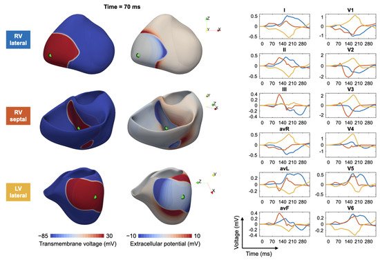
Figure 3 shows, as an example, a fast simulation of the spread of depolarization (transmembrane voltage and epicardial potentials) and the corresponding 12-lead ECG for three different ventricular extrasystoles.
Figure 3. Modeling of ectopic beats and the corresponding ECG: for three different trigger locations in the right ventricle (RV) and left ventricle (LV), the transmembrane voltage (left column), the extracellular potentials (middle column) and corresponding ECGs (right column) are shown. Excitation propagation was computed by solving the anisotropic Eikonal equation.