1. Introduction
Climate is a major driving factor for the distribution of the global forest ecosystem
[1]. Climate, especially temperature and precipitation, varies along latitude and continental position
[2]. Based on temperature and precipitation, the Köppen–Trewartha classification has divided global climate into six groups: tropical, dry climate, sub-tropical, temperate, boreal, and polar climate
[3]. Besides this, altitude also creates a mountain system which is defined by a minimum elevation of 300 m and minimum slope of 2° over 25 km
[4]. The mountain system contains distinct thermal belts, which are distinguished into a mountain (>15 °C), montane (6.4–10 °C), alpine (3.5–6.4 °C), and Nival belts (<3.5 °C)
[5]. In the broader context, the mountain system can be grouped into three belts: montane belt, alpine belt, and Nival belt. Likewise, the mountain system of Nepal is also divided into six life zones according to altitude: tropical (<1000 m), subtropical (1000–2000 m), temperate (2000–3000 m), subalpine (3000–4000 m), alpine (4000–5000 m), and nival zone (>5000 m)
[6].
The mountain system provides a wide array of ecosystem services. Around 20% (1.2 billion) of the world’s population resides in mountains areas and around half of humankind depends on mountain resources
[7]. Mountains sustain the lowland river discharge with varying degrees through glacial melting. Besides this, the mountain system sustains plant life up to the alpine belt, termed as an alpine ecosystem and referred to the communities found above the tree-line elevation. The alpine ecosystem covers 3% of the global land area. Because the alpine ecosystem is limited by distinct climate factors, viz. low temperature, low rainfall, strong winds, high solar radiation, low atmospheric pressure, and short growing season, there are great concerns that climate change will adversely affect this as well as the whole mountain ecosystem.
The mountain system of Nepal has distinct characteristics where the variation of topography exists from lowland warm and humid subtropical climate to high altitude climate with freezing temperature
[6]. The warm summer temperature in lowlands is around 22–27 °C, and there are high altitude regions with temperatures of 5–15 °C around Nepal. The precipitation of Nepal is dominated by the southeast tropical easterly monsoon from the Bay of Bengal. The Himalayas act as a cooling barrier which results in orographic precipitation in the summer season. The summer monsoon accounts for around 79.6% of the total precipitation of Nepal
[8]. The winter monsoon of Nepal is associated with a sub-tropical westerly jet from the northeast direction and comprises around 3.5% of total precipitation. Consequently, the summer monsoon sustains the summer streamflow of Nepal, whereas the winter streamflow largely depends on snow and glacier melt
[8]. Hence, temperature and precipitation are crucial for determining soil moisture, evaporation, streamflow, and snow cover. Besides this, the mountain system of Nepal comprises the world’s highest alpine ecosystem including the Everest region with elevation up to around 9 km above mean sea level. At present, the Everest region falls under Sagarmatha National Park. This region is recognized as the site of international importance (World Heritage Site, a conservation hotspot among WWF global 200 ecoregions, and a Ramsar site (Gokyo Lake)). The Everest region has an estimated 1074 species of flora and 247 species of fauna
[9]. This region is the water source of the Dudh Koshi River that sustains 0.46 million people on the Dudh Koshi river basin
[10]. In addition, the Dudh Koshi River possesses a hydropower potential of 2741.5 MW
[11]. Consequently, the changes in temperature and precipitation upstream in the high elevation of the Everest region are linked with the livelihood of the Dudh Koshi river basin. Hence, the study of the highest alpine ecosystem is essential to analyze the existing situation and manage the future potential risk.
In recent decades, the climate change issue has been a widespread concern all around the globe
[12]. A previous study indicated that Nepal Himalaya was experiencing high warming trend during 1935–1975
[13]. It is affirmed that alpine ecosystems are facing increasing warming and are greatly vulnerable to ongoing climate change as they are controlled by low temperatures
[14]. Using a variety of tools and techniques including satellite-based NDVI, climate change and its impacts have been observed across the Himalayas of Asia
[15][16][17][18][15,16,17,18]. These impacts include the expansion of alpine vegetation towards higher altitudes in Hindu Kush Himalaya
[19] and the conversion of alpine meadows to shrublands in the Tibetan Plateau
[20][21][20,21]. It is also reported that the shift in the alpine tree line is associated with a significant increase in air temperature in Western Himalayas, India
[22]. However, there are results of studies showing different responses of vegetation to climate change, suggesting that these are site specific, and the responses are modified by local drivers. For example, a study of the Tibetan Plateau showed that temperature is rising, but the vegetation greening rate decreases along elevation gradients
[16]. Similarly, a study of the entire Himalayas showed that most Himalaya regions show a greening trend, but, in the Eastern Himalayas, the vegetation shows a decreasing trend along with elevation
[23]. Specific to the Nepal Himalaya, unfortunately, the analysis of vegetation dynamics in relation to changes in climate variables is still lacking.
Besides vegetation, climate warming has also been found to affect cryospheric processes (such as changes in snow cover and glacier permafrost) and related hydrological processes (such as water cycle and balance and river discharge)
[7]. For example, globally, it was reported that during 1990–2018 the number and area of glacial lakes have rapidly increased from 9414 (5930 km
2) to 14,394 (8950 km
2), and the glacial lake volume has increased from 105.7 to 156.5 km
3 [24]. Similarly, the increasing number and area of glacier lakes were also revealed in the central Himalayas region during 1990–2010
[25]. At the scale of Nepal Himalaya, the number and area of glacier lakes have increased from 606 (55.53 km
2) to 1541 (80.95 km
2) from 1977 to 2017
[26]. It was revealed that the glacier has retreated at the rate of 10–59 m/year in the Everest region
[27]. The changes in the glacial lakes will favor vegetation growth by increasing the soil moisture and temperature. However, the glacial lakes at a higher altitude create a threat of glacial lake outburst flood (GLOF) to lowland people. Hence, the trend of glacial lake expansion by area and volume should be monitored on a long-term basis.
Although there are some studies on the vegetation dynamics Koshi river basin, and over Nepal, the study of high altitude forest ecosystem in response to climate change is still unexplored. This region has less human disturbance for land-use change because of extreme climate. Because of this, the alpine ecosystem is considered a quick indicator of the impacts of climate change. The long-term analysis of alpine vegetation of the Everest region will provide a better understanding of climate change interaction with high altitude. In addition, the trend analysis of the number and area of glacial lakes over a long-term basis is also new and useful for the prediction of water stress, adaptability, vulnerability, and overall water resource management in Nepal Himalaya. Specifically, to understand the relationships between climate variables and their potential impacts on the Everest region of Nepal, this study aimed to answer three research questions: (i) What are the trends of temperature and precipitation in the Everest region? (ii) What are the trends of glacial lake and streamflow changes in the Everest region? (iii) What are the NDVI trends and areal changes of alpine vegetation in the Everest region?
2. Analysis on Results
2.1. Trends in Climate Variables
2.1.1. Temperature Trend
The results of the modified Mann–Kendall test for annual and seasonal temperature data for 1995–2019 are presented in
Table 12. A positive
z-value (
Table 12) and slope value (
Figure 14 and
Table 23) indicate an increasing trend, whereas a negative
z-value and slope value indicate a decreasing trend. The Kendall’s tau value explains the strength of correlation between variables, ranging from −1 to +1. Annual and seasonal temperature trends based on the linear regression method are shown in
Figure 14 and
Table 23. Significances are provided at 90%, 95%, and 99% confidence levels.
Figure 14. Linear regression trends of annual temperatures.
Table 12. Summary of the modified Mann–Kendall statistical tests of temperature trend.
| Series |
Mean Temperature |
Maximum Temperature |
Minimum Temperature |
| z-Value |
Tau |
p |
z-Value |
Tau |
, the mean annual temperature, maximum annual temperature, and minimum annual temperature show significant increasing trends. The magnitude of trends for mean, maximum, and minimum annual temperatures are 0.0329, 0.0415, and 0.055 °C/year, respectively.
In addition, summer maximum temperature and summer minimum temperature show significant increasing trends of 0.0343 and 0.0341 °C/year, respectively. The winter maximum temperature and winter minimum temperature show higher significant increasing trends of 0.078 and 0.0915 °C/year, respectively. This shows that winter warming is around 2.5 times faster than summer warming. Similarly, an insignificant but coherent warming trend is also found in spring. Autumn maximum temperature and autumn minimum temperature show warming trends of 0.0358 and 0.0467 °C/year, respectively.
Since ERA5 reanalysis data are interpolated data, they were again compared with the nearest observation data by the independent
t-test. The results are shown in
Table 34. We found that there is no significant difference between the mean of reanalysis and observation data.
Table 34. Summary of the independent t-test results of reanalysis versus observation annual temperature data.
| Year |
Mean Temperature
(Reanalysis vs. Observation) |
Max. Temperature
(Reanalysis vs. Observation) |
Min. Temperature
(Reanalysis vs. Observation) |
| t-Value | p |
p-Value | z-Value |
zTau |
p |
| t | -Value |
p-Value |
t-Value |
p-Value |
|---|
| Winter |
1.91 |
0.20 |
0.06 |
1.66 |
0.24 |
0.10 |
2.1.2. Precipitation Trend
As indicated in
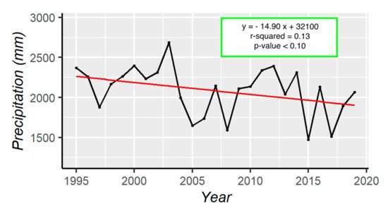
Table 45, the annual precipitation shows a decreasing monotonic trend at a 95% confidence level. Winter and autumn precipitation show the existence of a monotonic trend at a 95% confidence level. With a 90% confidence level, summer precipitation also shows a negative monotonic trend. The negative
z-value and tau value indicate the decreasing trend. In
Figure 25, a significantly decreasing trend with a 90% confidence level is observed in the annual precipitation series. The magnitude of the trend is −14.90 mm/year.
Figure 25. Linear regression trends of annual precipitation.
Table 45. Summary of the modified Mann–Kendall statistical tests of precipitation, glacial lake area, and mean NDVI.
| Series |
Precipitation |
Glacial Lake Area |
Mean NDVI |
| z-Value |
Tau |
p |
z-Value |
Tau |
p |
z-Value |
-ValueTau |
p |
| Tau |
p |
| 3.18 |
0.29 |
<0.01 |
| Spring |
| Winter |
| Winter |
−2.44y = 0.0579x − 123 |
−0.27R2 = 0.08 |
0.01ns |
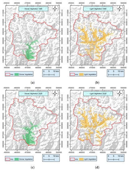
) light vegetation 1995; (c) dense vegetation in 2020; (d) light vegetation in 2020.
To check the classification accuracy, 75 random sample points for dense vegetation were examined by field observation and 75 random sample points for light vegetation were examined by Google Earth imagery (
Figure 3). Then, the confusion matrix was created, which showed that the overall classification accuracy is 76.33% for the classified image. The classification accuracy for the dense vegetation is 89%, whereas the classification accuracy of light vegetation is 72% (
Table 67). The overall Kappa coefficient for 2020 is 0.76.
Table 67. Confusion matrix for the referenced and classified dataset.
| |
Reference Data Set |
User’s Accuracy |
| Land Cover |
Dense Vegetation |
Light Vegetation |
Other Classes |
Total |
| 1.64 |
0.24 |
0.10 |
2.23 |
0.45 |
| Winter |
1.24 |
0.18 | 0.03 |
0.22 |
| Classified data set |
Dense Vegetation | <0.01 |
<0.01 |
1.00 |
0.07 |
610.01 |
0.95 |
0.54 |
0.08 |
0.59 |
1.08 |
0.16 |
0.28 |
1.91 |
0.27 |
| Spring | 0.06 |
| 0 |
0 |
61 |
100 |
0.74 |
0.09 |
0.46 |
1.29 |
Spring0.18 |
−4.310.20 |
−0.36 |
<0.01 |
| Light Vegetation |
14 |
54−3.51 |
−0.31 |
Summer |
3.79 |
0.54 |
<0.01 |
Autumn |
1.13 |
0.18 |
0.26 |
| Spring |
y = 0.0178x − 35.60 |
R2 = 0.02 |
ns |
2.67 |
0.38 |
0 |
68 |
79.410.01 |
<0.01 |
−2.43 |
−0.35 |
0.02 |
3.29 |
0.47 |
<0.01 |
3.12 |
| Summer |
−2.34 |
−0.47 |
1.97 |
0.28 |
0.05 |
1.41 |
| Summer | 0.45 |
y = 0.0287x − 49.40 |
R2 = 0.46 |
***<0.01 |
| Summer |
0.02 |
0.54 |
0.08 |
0.59 |
−3.06 |
−0.44 |
0.22 |
0.16 |
| <0.01 |
| Other Classes |
0 |
21 |
Autumn |
y = 0.0279x − 53.60 |
Autumn | R2 = 0.09 |
ns |
−3.71 |
−0.44 |
Annual |
1.78 |
0.26 |
0.07 |
2.27 |
0.33 |
0.02 |
2.46 |
0.35 |
0.01 |
Summary of the modified Mann–Kendall statistical tests of temperature trend.
Table 23. Linear regression equations of all seasonal series of temperature, precipitation, streamflow, NDVI, and surface water area.
| Climate Variables |
Season Variables (y) |
Regression Line |
R2 |
p-Value |
| Mean Temperature |
| <0.01 |
−0.47 |
−0.07 |
0.64 |
<0.01 |
<0.01 |
1.00 |
| Maximum Temperature |
Winter |
y = 0.078x − 157 |
R2 = 0.13 |
* |
| −1.71 |
−0.20 |
0.09 |
0.90 |
0.10 |
0.37 |
2.42 |
0.30 |
0.02 |
| Autumn |
−2.06 |
−0.32 |
0.04 |
3.69 |
| Annual |
−2.87 |
−0.41 |
<0.01 |
−0.58 |
−0.09 |
0.56 |
−3.29 |
−0.47 |
<0.01 |
Summary of the modified Mann–Kendall statistical tests of streamflow.
2.3. Alpine Vegetation
2.3.1. Spatial Change Detec2tion
Alpine vegetation represents life at climate limits and is a quick indicator of climate change. Based on GIS analysis, around 97.5% of the study area is a high-altitude region having an elevation of more than 3000 m. Thus, alpine vegetation in the Everest region mostly possesses alpine grasses, juniper shrubs, and conifer forests.
Figure 58 shows the vegetation maps in 1995 and 2020. It is observed that the dense vegetation increased from 103.5 to 150 km
2 (45% increase), while light vegetation shows minor changes, increasing from 300.2 to 303.4 km
2. This result shows the most marked expansion in dense vegetation in the Everest region. On the other hand, despite the constant areal extent, light vegetation such as alpine meadows/rangeland and juniper scrubs also shows expansion towards upper altitude, as shown in
Figure 58.
Figure 58. Alpine vegetation: (a) dense vegetation in 1995; (b
| 21 |
| 100 |
| Total |
75 |
75 |
0 |
150 |
|
| Producer’s Accuracy |
89.00 |
72.00 |
0 |
|
76.33 |
Confusion matrix for the referenced and classified dataset.2.3.2. NDVI Change Detection
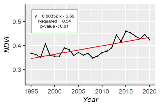
The result of the modified Mann–Kendall test for NDVI is shown in
Table 45. It is revealed that there is a significant increasing trend in annual NDVI at a 95% confidence level. Similarly, all seasonal NDVI trends are also increasing significantly at a 95% confidence level.
Figure 69 and
Table 23 show the linear regression trend of annual and seasonal NDVI during 1995–2019. It is noted that the NDVI is increasing at a rate of 0.0035 units/year. Seasonally, the autumn NDVI shows the highest increasing rate of 0.0051 units/year. More importantly, the spring growing season also shows a significant increasing trend. An abrupt rise in annual NDVI was observed in 2008. This also indicates the greening trend is increasing in the Everest region.
Figure 69. Linear regression trends of NDVI.
2.4. Alpine Region Change and Its Relationship with Climate Variables
The responses of alpine vegetation (NDVI) and surface water (glacial lake area plus streamflow) are analyzed by the multiple linear regression method (
Table 78). Here, the temperature and precipitation variables are considered as independent (
x) variables, while the NDVI, surface water, and streamflow are considered as dependent (
y) variables.
Table 78. Multiple linear regression equations for the relationship between alpine vegetation (NDVI) and surface water (glacial lake plus streamflow) with temperature and precipitation.
| Response Variables (y) |
Multiple Regression
Equations |
Seasonal Variables (xij) |
R2 |
Significance |
| Annual NDVI |
y1 = −0.2869 x1 + 0.0977 x2 + 0.1596 x3 + 0.672 |
x1 = annual mean temperature,
x2 = annual maximum temperature,
x3 = annual minimum temperature |
R2 = 0.65 |
*** |
| Annual NDVI with seasons |
y1 = −0.2252 x14 + 0.1262 x24 + 0.0944 x34 + 0.00004 x43 + 0.0004 x44 |
x14 = autumn mean temperature,
x24 = autumn maximum temperature,
x34 = autumn minimum temperature
x43 = summer precipitation,
x44 = autumn precipitation |
R2 = 0.94 |
*** |
| Winter NDVI (y11) |
y11 = −0.0003 x42 |
x42 = spring precipitation, |
R2 = 0.92 |
*** |
| Summer NDVI (y13) |
y13 = −0.2900 x14 − 0.5767 x22 + 0.2117 x24 − 0.0003 x42 − 0.00008 x43 + 0.0008 x44 |
x14 = autumn mean temperature,
x22 = spring maximum temperature,
x24 = autumn maximum temperature,
x42 = spring precipitation,
x43 = summer precipitation,
x44 = autumn precipitation |
R2 = 0.89 |
** | 0.53 |
<0.01 |
3.67 |
0.53 |
<0.01 |
| Autumn NDVI (y14) |
y14 = −0.1673 x23 |
x23 |
Spring |
y = 0.0181x − 31.50 |
R2 = 0.02 |
ns |
| Summer |
y = 0.0343x − 57.80 |
R2 = 0.40 |
*** |
| Autumn |
y = 0.0358x − 65 |
R2 = 0.17 |
** |
| Minimum Temperature |
Winter |
| R |
| Annual |
−2.37 |
−0.26 |
0.02 |
2.87 |
= summer maximum temperature |
R2 = 0.910.39 |
**<0.01 |
2.01 |
| Surface water |
y2 = 1.0399 x3 − 0.0114 x4 |
x3 = annual minimum temperature
x4 = annual precipitation |
R2 = 0.71 |
*** |
Glacial lake area
at summer (y23) |
y |
y = 0.0915x − 196 |
R2 = 0.14 |
* |
| Spring |
y = 0.0482x − 102 |
R2 = 0.10 |
ns |
| 23 = −0.0023 x43 |
x43 = summer precipitation |
R2 = 0.82 |
*** |
Glacial lake area
at autumn (y24) |
y24 = −4.1189 x11 + 2.0369 x21 − 3.0521 x22 − 0.0162 x44 |
x11 = winter mean temperature,
x21 = winter maximum temperature,
x22 = spring maximum temperature,
x44 = autumn precipitation |
R2 = 0.93 |
*** |
Spring average
streamflow (y32) |
y32 = 165.0526 x32 + 0.6938 x44 |
x32 = spring minimum temperature,
x44 = autumn precipitation |
R2 = 0.69 |
ns |
Summer average
streamflow (y33) |
y33 = −838.3610 x24 |
x24 = autumn maximum temperature, |
R2 = 0.76 |
ns |
Summer |
| Spring maximum | y = 0.0341x − 62.90 |
streamflow (y42) |
y42 = -131.2207 x12 + 111.2719 x32 -148.4615 x | R2 = 0.38 |
*** |
| 34 |
x12 = spring mean temperature,
x32 = spring minimum temperature,
x34 = autumn minimum temperature |
R2 = 0.75 |
ns |
Autumn |
Autumn maximum
streamflow (y44)y = 0.0467x − 95.50 |
y44 = 1.8552 x44R2 = 0.14 |
x* |
| 44 | = autumn precipitation |
R2 = 0.79 |
ns |
Precipitation |
Winter |
y = −1.49x + 3030 |
Annual minimum
streamflow |
y5 = −75.6473 x1 − 52.0933 x3 | R |
x1 = annual mean temperature,
x3 | 2 = 0.06 |
ns |
| = annual minimum temperature |
R | 2 = 0.50 |
*** |
Spring |
y = 0.973x − 1750 |
R2 = 0.02 |
Winter minimum
streamflow (y51) | ns |
| y51 = 1.8552 x44 |
x44 = autumn precipitation |
R2 = 0.68 |
ns |
Summer |
y = −12x + 25,800 |
R2 = 0.09 |
Spring minimum
streamflow (y52) |
y52 = −99.7734 x41 − 0.1012 x42 + 0.2165 x44 |
x42 | ns |
| = spring precipitation, |
| x44 = autumn precipitation |
R2 = 0.83 |
ns |
Autumn |
y = −2.46x + 4990 |
Summer minimum
streamflow (y53) | R2 = 0.11 |
ns |
| y53 = 636.6429 x14 − 317.3432 x24 |
x41 = winter precipitation,
x14 = autumn mean temperature,
x24 = autumn maximum temperature, |
R2 = 0.73 |
ns |
Average Streamflow |
Winter |
y = 0.29x − 534 |
R2 = 0.09 |
ns |
| Spring |
y = −2.64x + 5440 |
R2 = 0.22 |
** |
| Summer |
y = −11.4x + 23,400 |
R2 = 0.34 |
*** |
| Autumn |
y = −2.48x + 5110 |
2 = 0.35 |
*** |
| Maximum Streamflow |
Winter |
y = 0.0713x − 87.60 |
R2 ≤ 0.01 |
ns |
| Spring |
y = −1.07x + 2230 |
R2 = 0.10 |
ns |
| Summer |
y = 1.05x − 1080 |
R2 ≤ 0.01 |
ns |
| Autumn |
y = −2.19x + 4630 |
R2 = 0.02 |
ns |
| Minimum Streamflow |
Winter |
y = 0.0779x − 115 |
R2 = 0.01 |
ns |
| Autumn |
y = −0.656x + 1350 |
R2 = 0.22 |
** |
| Summer |
y = −4.76x + 9800 |
R2 = 0.39 |
*** |
| Autumn |
y = −0.0455x + 182 |
R2 ≤ 0.01 |
ns |
| Mean NDVI |
Winter |
y = 0.00338x − 6.45 |
R2 = 0.48 |
*** |
| Spring |
y = 0.00309x − 5.87 |
R2 = 0.32 |
*** |
| Summer |
y = 0.0026x − 4.76 |
R2 = 0.25 |
*** |
| Autumn |
y = 0.00506x − 9.74 |
R2 = 0.54 |
*** |
| Glacial Lake Area |
Winter |
y = 0.0784x − 154 |
R2 = 0.19 |
** |
| Spring |
y = 0.045x − 87.40 |
R2 = 0.10 |
ns |
| Summer |
y = 0.0346x − 63.90 |
R2 = 0.07 |
ns |
| Autumn |
y = 0.151x − 295 |
R2 = 0.43 |
*** |
Linear regression equations of all seasonal series of temperature, precipitation, streamflow, NDVI, and surface water area.
In
Table 12, the maximum annual temperature and minimum annual temperature trends show the existence of a monotonic trend at a 95% confidence level. Similarly, the mean annual temperature also shows the existence of a monotonic trend at a 90% confidence level. Besides, all the positive tau values and
z-values in
Table 12 indicate that the temperature is positively correlated or increasing with time series. As shown in
Figure 4, variations from years to years are common in temperature trends but all indicate the warming trends. The maximum and minimum annual temperature trends are increasing significantly at a 95% confidence level, whereas the mean annual temperature trend shows a significant positive trend at a 90% confidence level. Similarly, the significant increasing trend is shown in the summer season of mean, maximum, and minimum temperature at a 99% confidence level (
Table 12). According to the linear regression test shown in
Figure 14
| 1995 |
−1.23 |
0.23 |
−1.15 |
0.26 |
−0.86 |
0.40 |
Summary of the independent t-test results of reanalysis versus observation annual temperature data.
Summary of the modified Mann–Kendall statistical tests of precipitation, glacial lake area, and mean NDVI.
2.2. Surface Water
2.2.1. Glacial Lake Changes
The results of the modified Mann–Kendall test for annual and seasonal data are shown in
Table 45. It is observed that the annual surface water extent in the Everest region shows a positive monotonic trend at a 95% confidence level.
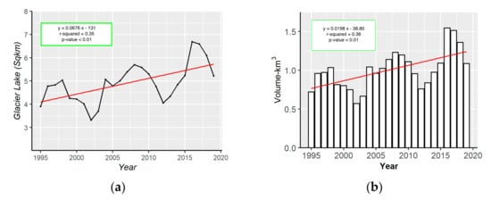
The seasonal and annual surface water extent trends based on the linear regression test are shown in
Table 23 and
Figure 36a. We found that the surface area of glacial lakes is increasing at the rate of 0.068 km
2/year. The significant increasing trend is shown at a 99% confidence level. Based on the season, winter and autumn seasons show an increasing rate of 0.078 and 0.15 km
2/year, respectively (
Table 23). The average surface area of glacier lakes in the study area is 4.9 km
2. Thus, this observed increasing rate is quite significant. In
Figure 36b, the glacial lake volume also shows a significant increasing trend with a rate of 0.0198 km
3/year. The average glacial lake volume is 1.01 km
3.
Figure 36. Glacial lake: (a) change in surface area; (b) changes in lake volume.
2.2.2. Streamflow Trend
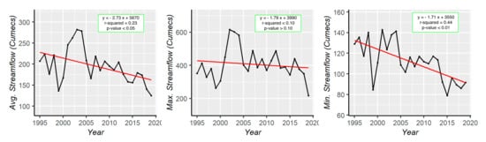
According to the streamflow data for 1995–2015 recorded at Rabuwa Bazar gauging station, the maximum flowing rate is 2580 m
3/s (cumecs), the minimum flowing rate is 9.07 m
3/s, and the average flowing rate is 199 m
3/s. The results of the modified Mann–Kendall test for annual and seasonal data are shown in
Table 56 and
Figure 47. In
Table 56, it is observed that a significant decreasing trend is found in average annual streamflow and minimum annual streamflow at a 95% confidence level. The magnitudes of trend in average annual streamflow and minimum annual streamflow are −2.73 and −1.71 m
3/s/year, respectively. It is also seen that the average summer streamflow and average minimum streamflow show significant decreasing trends. However, most of the trends for the maximum seasonal streamflow were not statistically significant. Similarly, all the spring season streamflows show significant decreasing trends.
Figure 47. Linear regression trends of annual streamflow.
Table 56. Summary of the modified Mann–Kendall statistical tests of streamflow.
| Series |
Average Streamflow |
Maximum Streamflow |
Minimum Streamflow |
| z-Value |
Tau |
p |
z-Value |
Tau |
p |
Multiple linear regression equations for the relationship between alpine vegetation (NDVI) and surface water (glacial lake plus streamflow) with temperature and precipitation.
The table shows that 65% of the annual variability of NDVI is explained by mean, maximum, and minimum annual temperature. Further, regarding the seasonal variability, autumn temperature and summer precipitation explain 94% of the variability of annual NDVI. Similarly, 71% variability of surface water extent is represented by minimum annual temperature and annual precipitation. Overall, there is a high level of confidence that alpine vegetation and temperature are strongly correlated.
3. CDiscurrent Insightsssion
3.1. Climate Trend
Temperature, precipitation, and solar radiation are the major climate controls that act as limiting factors for vegetation growth
[28][54]. Some studies found that temperature is responsible for 31–33% of Earth’s vegetation growth; precipitation is responsible for 40–52% of vegetation growth; solar radiation is responsible for 5–27% of vegetation growth
[28][29][54,55]. In this study, it is revealed that the annual mean, maximum, and minimum temperatures at the Everest region are increasing at the rates of 0.0329, 0.0415, and 0.055 °C/year, respectively. In line with this result, Shrestha et al.
[13] also found that the maximum temperature is increasing rate at 0.057 °C/year in the entire Nepal Himalayas. Within seasonal temperature, winter maximum temperature and winter minimum temperature show higher warming trends than the summer season. On the global scale, it is observed that winter warming is faster than summer warming
[30][56]. Winter warming is ecologically more crucial. Winter warming can promote vegetation growth by reducing the seasonal frost of the winter season
[31][57]. An experiment has discovered that soil respiration is increased by 9.3% by winter warming
[32][58]. Winter warming stimulates litter decomposition in the winter season. Most importantly, prolonged winter warming triggers advancement in spring plant phenology and eventually increases the length of the growing season
[33][59]. On the other hand, the annual precipitation of the Everest region shows a decreasing monotonic trend. However, the magnitude of change is found at −14.90 mm/year at a 90% confidence level. Besides this, summer precipitation also shows a decreasing trend at a 90% confidence level. Salerno et al.
[34][60] also observed that the monsoon precipitation was weakening (−9.3 mm/year) in the Everest region during 1994–2013. Another larger-scale study including the Everest region by Shrestha et al.
[35][61] found an increasing annual precipitation over the entire Koshi river basin (area of 87,970 km
2) from 1975 to 2010. However, this study did not include the stations in the study area, and the results in this study might be due to local spatial variation. Hence, the climate condition of the Everest region has changed over the recent 25 years period. This climate change is very likely to alter the alpine ecosystem and cryospheric processes of the Everest region.
3.2. Surface Water Dynamics
It is estimated that the glaciers are decreasing an average of 267 Gt/year at the global scale and 6 Gt/year in South Asia
[36][62]. As a result, glacial lakes are growing. In the Everest region, the result shows the increasing trend of glacial lake surface area at 0.0676 km
2/year. The glacial lake volume has been increasing at the rate of 0.0198 km
3/year. Bajracharya et al.
[37][63] also found that the moraine-dammed lakes’ area, that is lakes formed due to blockade glacier debris, in the Dudh Koshi river basin increased from 2.291 to 7.254 km
2 between 1996 and 2000. Similarly, Salerno et al.
[38][64] found that the number and area of glacier lakes in the Everest region especially in the designated area of Sagarmatha National Park have increased. They reported 624 glacial lakes with an area of 7.43 km
2 in 2008. The reason behind the glacial lake changes might be linked to temperature and precipitation change. A study of the Tibetan Plateau also found that the glacial lake expansion is highly correlated with glacier area recession, and this variation is associated with temperature rising
[39][65]. The Everest region is also facing significant temperature rising, especially winter warming. Moreover, the glacial lake expansion may foster positive and negative impacts. There are unique glacier ecosystem services such as irrigation and drinking water supply to the downstream population and lowland discharge. However, most glacial lakes are formed by blockade of ice, glacier debris, landslide, and are inherently unstable type and susceptible to glacial lake outburst floods. Future endeavors should therefore be given to the study of glacial lake water resource utilization and their risk management.
Similarly, the average annual streamflow of the Dudh Koshi river basin is 199 m
3/s. Dudh Koshi is a tributary of the Koshi River. The average flow of the Koshi River is 1658 m
3/s. Similarly, the average flow of the three other major river basins of Nepal, namely, Gandaki, Karnali, and Mahakali, are 1753, 1441, and 698 m
3/s, respectively
[40][66]. In this study, from 1995 to 2019, we observed that the average annual streamflow is decreasing at the rate of 2.73 m
3/s/year. These decreasing flow trends are consistent with weaker precipitation in the Everest region. Besides, the temperature is increasing, which might trigger more precipitation in the Everest region, but this is not the case. Gautam and Acharya
[41][67] found a decreasing trend in the streamflow of the Dudh Koshi River basin from 1967 to 1997. Hence, the streamflow of the Dudh Koshi River is declining, which causes a water availability risk to the river-dependent ecosystems and societies. In addition to the need to closely monitor glacial lakes as mentioned above, it is also urgent and essential to evaluate the potential water stress associated with decreasing precipitation in this river basin.
3.3. Alpine Vegetation Dynamics
In this study, we found that NDVI is increasing at a rate of 0.00352 units annually. All the seasonal NDVIs are increasing with the highest in the autumn season. We also observed that annual NDVI is associated with autumn warming. Shi et al. found that autumn warning delays the end of the plant growing season for deciduous forests
[42][68]. However, the study area consists of mostly evergreen conifer forests and perennial shrubs. Autumn warming also promotes vegetation growth by reducing frost damages
[43][69]. The prominent increase in autumn NDVI reflects the increase in the extent of perennial vegetation. Additionally, the significant winter warming in the Everest region also favors vegetation growth. It is assessed that the dense vegetation cover has increased from 103.5 to 150 km
2. Consistent with this, Baniya et al.
[17] also observed a greening trend in all of Nepal with significant NDVI trends at 0.0005 and 0.002 units/year in the spring and autumn season, respectively. The driving factors for these increasing trends are attributed to temperature (39.62%), ecological restoration (25.16%), and multiple factors (35.22%). Over the larger scale in the Koshi river basin, Wu et al.
[18] found a greening trend of 0.0023 units/year from 2000 to 2018. Zhang et al.
[15] also showed the increasing rate of average growing season NDVI over the Koshi River basin at the rate of 0.0034 units/year from 2000 to 2011. In the context of greening in the Everest region, there might be multiple casual/control factors. The greening trend is increasing despite weaker precipitation. The ecological restoration program was also held in the study area. However, the area of the plantation during 1979–2008 is small (1.51 km
2) as compared to the increasing area
[9]. Ecological restoration in the Everest region is also challenging because of less water, cold weather, and rocky topography. Besides, the Everest region had around 1.02 km
2 settlement area and 8.50 km
2 agriculture area in 2011, and this region is managed under park regulations. Hence, the human disturbances to land-use change are considered minimal
[44][28]. The shrub promotion due to overgrazing and abandonment of remote farmland is likely to favor vegetation expansion. Hence, it is obvious that the vegetation expansion is also driven by climatic factors. In this study, we found that annual NDVI is highly correlated with annual temperature. The abrupt rise of annual NDVI during 2008–2015 coincided with an increasing trendline in annual mean temperature during 2003–2009. Moreover, the annual precipitation showed an increasing trendline during 2008–2012 despite weak precipitation over the period. Furthermore, the temperature change can drive an upper shift in snow line altitude, which subsequently favors temperature for vegetation expansion and migration
[45][70]. It is also revealed that temperature triggered alpine vegetation greening on the Tibetan Plateau from 1982 to 2011
[46][71]. For future endeavors, long-term research on phenological changes and carbon dynamics of the alpine vegetation may explore more about the climate change impacts on the high-altitude region.