Your browser does not fully support modern features. Please upgrade for a smoother experience.
Please note this is a comparison between Version 1 by David Morgan and Version 2 by Amina Yu.
The surface chemistry of carbon materials is predominantly explored using x-ray photoelectron spectroscopy (XPS). However, many journal articles have critical failures in the published analysis which typically stems from an ill-informed approach to analyzing the spectroscopic data. The presented work presents a discussion on lineshapes and associated changes in the spectral envelope of predominantly graphitic materials, which together with the use of the D-parameter to verify levels of the graphitic content, using this information to highlight a simple and logical approach to strengthen confidence in the functionalization derived from the carbon core-level spectra.
- carbon
- XPS
- oxygen
- fitting
- quantification
1. Introduction
The chemistry of carbon materials is extremely important in fields such as catalysis, energy storage, composite materials, and sensor technology to name but a few examples [1]. In the analysis of such materials, to obtain an understanding of the surface properties the use of x-ray photoelectron spectroscopy (XPS) has been ubiquitous due to its inherent surface sensitivity. Given the truly heterogenous nature of most carbons, with their bonds to hetero atoms, different chemical species, and varying amounts of sp2 and sp3 carbon, the carbon spectral envelope can become quite convoluted.
Many researchers approach the analysis of carbon from a single point of view, specifically analysis of solely the C (1s) region. Complementary analysis of the corresponding heteroatom spectral regions (e.g., O (1s), S (2p), and N (1s)) is required to support the conclusions drawn by the C (1s) analysis [2][3][4][5][2,3,4,5].
Erroneous analysis also stems from failure to apply an asymmetric shape to graphitic carbon, which arises from final-state effects due to the photoelectron ejection [6][7][8][9][6,7,8,9], while a failure to consider the presence of defects or changes in the electronic structure of the carbon can also lead to mistaken assignments of peaks in a fitting model.
This paper reviews and addresses some of the key points that are commonly made in error in the published literature, including photoemission line shapes, the use of the carbon Auger and simple checks a researcher can perform to move towards a better understanding of their carbon material and have confidence in their chemical state assignments from peak fitting.
2. The C (1s) Spectrum of Diamond, HOPG and Graphitic Carbons
This paper will not consider the fitting of adventitious or polymeric carbon species but will focus on predominantly graphitic and diamond-like materials. For discussion on the former, the reader is directed to [10][11].
Diamond, with its sp3 hybridization, typically exhibits a Voigt-like peak shape and is taken to have a binding energy of 285 eV [11][12][12,13]. The C (1s) core-level spectrum of graphitic carbon, such as that of HOPG, is characterized by an asymmetric peak shape with a binding energy typically reported as 284.5 eV (although values between 284.3 and 284.6 eV have been reported [11][13][12,14]) and a characteristic π-π* shake-up structure with structure centered around 291 and 294.5 eV (Figure 1).
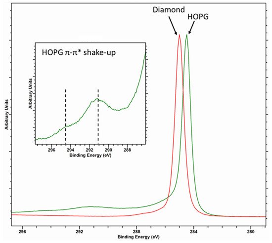
Figure 1. Overlayed C (1s) core level for diamond (red spectra) and HOPG (green spectra) with inset of the graphitic satellite structure.
The fitting of the graphitic C (1s) envelope is one of the most common errors encountered in the literature [14][15], and the asymmetric shape is something commonly ignored in may published papers. Recently, Linford et al. [10][11] reported a method for fitting the C (1s) envelope of graphitic carbon materials, using a reference spectrum of clean graphite/HOPG as a model for the graphitic backbone. This method is useful and is indeed a method the current author has used for many years. However, as shown in Figure 2, an apparently pure sp2 graphitic carbon (here a “nano-onion” [3]) cannot be fitted with the parameters taken from HOPG and likely stems from a combination of hydrogenation and the curvature of the carbon surface [13][14].
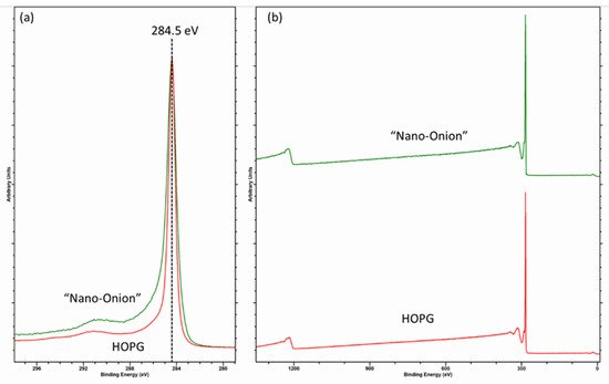
Figure 2. (a) C (1s) core-level and (b) survey spectra for HOPG, and hydrogenated “nano-onion” carbons illustrating the influence of hydrogenation on the C (1s) spectra.
Hydrogenation undoubtedly introduces some sp3 character given the broadening around 285 eV and accompanied by a reduction in the D-parameter (discussed in the following section) to 20.5. However, note the broadening with respect to the narrow HOPG spectrum, taking the difference spectra (not shown) shows some perturbation of the π-π* shake-up, which may be expected if there is a lattice disruption, accompanied with some broadening centered at 284.8 and 284 eV and are values consistent with Blume et al. [13][14] and assigned as disordered (thought to be due to random orientations of dangling bonds with respect to the carbon atoms) and defective carbon, respectively. Such defective induced broadening will cause a change in the main peak asymmetry due to screening of localized areas of charge and the need to adjust any asymmetric fitting parameters for the graphitic peak.
As will be shown in the following sections, analysis, especially fitting, of the C (1s) envelope for graphitic materials is complex and should not be fitted unless a rigorous and self-consistent model is used.
3. The C (KVV) Auger Peak and the D-Parameter
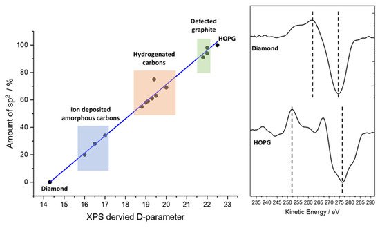
Not to be confused with the D-band in Raman spectroscopy of carbon materials, which is a measure of disorder of the graphitic material [15][16][17][16,17,18], use of the XPS-derived D-parameter to discriminate carbon states was demonstrated by Lascovich and co-workers [18][19][20][21][19,20,21,22], who showed a linear relationship existed between the extremes of pure sp2 and sp3 carbons by taking the first differential of the carbon Auger peak, where depending upon the relative concentrations of sp2 and sp3 carbon, the separation (D, hence D-parameter) of the differential maxima and minima differ greatly. Figure 3 shows a plot of the values of Lascovich et al. together with the first differential of the Auger peaks for diamond and HOPG. This approach has successfully been used to distinguish sp2 and sp3 rich carbon rich domains through XPS mapping experiments [22][23][23,24].
Consideration should be given in taking the D-parameter as an exact value, however. The electron kinetic energy of the Auger peak is lower than that of the C (1s) photoelectron kinetic energy (ca. 260 and 1200 eV, respectively), yielding an electron inelastic mean free path (IMFP) of 3.3 nm for the core-level photoelectron and 1.1 nm for the Auger electron—a threefold difference in electron depth and therefore a similar magnitude of difference in the XPS information depth [24][25]. The Auger electrons are more surface sensitive, hence sensitive to contamination. This is demonstrated by the data in Figure 4, where a freshly cleaved HOPG sample has been analyzed and then gently cleaned using an argon cluster source (operating at 4 kV, 2000 atoms); note how the C (1s) data are almost indistinguishable, while the Auger peaks differ significantly. The D-parameters here are 22 eV (cleaved) and 23.5 eV (cluster cleaned [25][26]), the latter being higher than that previously reported, while the former is in the range typically reported for graphite [11][12][18][19][20][22][26][12,13,19,20,21,23,27]; note none of these references mention in situ cleaning.
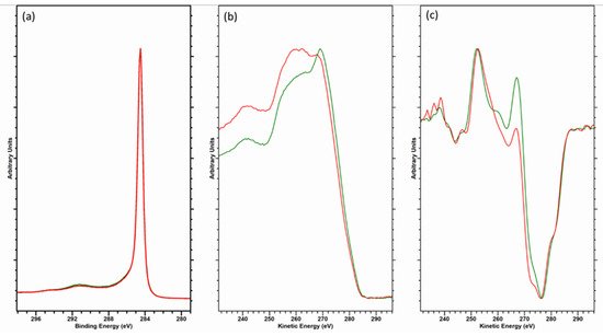
Figure 4. Overlayed data for (a) C (1s) core-level, (b) C (KVV) Auger and (c) first derivative C (KVV) spectra for freshly cleaved (red) and argon cluster cleaned (green) HOPG.
Irrespective of these values, there will be an uncertainty in the determination of the D-parameter depending on the method and parameters used. It is worth noting the C (KVV) Auger is typically recorded at a high pass energy, a step size of 0.5 eV and sufficient scans for a good signal-to-noise ratio (typically at least ×50) [27][28].
4. Conclusions
Using the logical approach and where applicable, parameters discussed herein, together with utilisation of the O(1s) spectrum in a complimentary manner, then an algorithmicized approach to fitting such as that shown in Figure 5, will lead to more reliable and meaningful chemical speciation being extracted from the C(1s) spectrum of the material for functionalized carbons and fullerene materials.
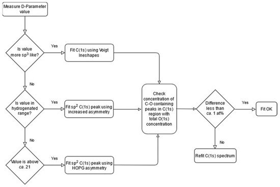
Figure 5. Methodology for the fitting of carbon materials described as a flowchart.