Your browser does not fully support modern features. Please upgrade for a smoother experience.
Please note this is a comparison between Version 1 by Di Zhang and Version 2 by Amina Yu.
Tilting Mapping Function (TMF) is a tropospheric mapping function to scale the slant tropospheric delays from various elevation and azimuth angles to the zenith direction. Based on the theory of tilting troposphere, TMF can represent the neutral atmosphere's asymmetry more accurately than traditional continued fraction mapping functions.
- tropospheric delay
- ray-trace
- mapping function
- tilting troposphere
- gradient
1. Introduction
Tropospheric delay refers to the effect caused by the propagation of the radio signals among the neutral atmosphere, which can be divided into a hydrostatic part and a wet part [1]. Many regional or global tropospheric delay models have been built to reduce the tropospheric delay error, which can be divided into two categories, depending on whether meteorological factors are needed or not [2]. Models of the first category use pressure, temperature, and humidity as their input parameters, such as Hopfield [3], Saastamoinen [4], Davis [5], Baby [6], Ifadis [7], Askne, Nordius [8], and MSAAS [9]. If in-situ meteorological observations are not available, the standard atmosphere [10][11][12][10,11,12] or empirical meteorological models [13][14][15][13,14,15] may also be used in many GNSS data processing applications. The second category doesn’t rely on meteorological measurements, such as UNB [16], MOPS [17], TropGrid [18], ITG [19], IGGTrop [20], and SHAtropE [21].
However, due to the irregular spatial and temporal distribution of water vapor, it is challenging to precisely model the wet part of the tropospheric delay. Thus it has been a commonly used strategy for Global Navigation Satellites Systems (GNSS) data processing to estimate the tropospheric zenith delay [22][23][24][22,23,24], especially for high precision applications [25][26][25,26]. The estimated Zenith Wet Delay (ZWD) can be converted into Precipitable Water Vapor (PWV) [27][28][29][27,28,29], and therefore GNSS meteorology has gradually become a fundamental and effective method for sounding the atmosphere under any weather condition. Barriot, et al. [30] proposed an approach based on perturbation theory, with the ability to separate eddy-scale variations of the wet refractivity.
The mapping function has been used to scale the slant delays from various elevation angles to the zenith direction. Consequently, the mapping function’s accuracy has significant and direct impacts on the determination of the ZWD and station coordinate. Since Marini first proposed the continued fraction form [31], almost all modern mapping functions, including Ifadis [7], MTT [32], NMF [33], IMF [34], UNBabc [35], VMF [36], GMF [37], VMF1 [38], GPT2 [39], and VMF3/GPT3 [40], have taken it as their model expression. Each mapping function has two subtypes: the hydrostatic part and the wet part. The main difference among various mapping functions is the specific value of each coefficient.
However, the Marini concept mapping functions were built on the assumption of the neutral atmosphere’s spherical symmetry [41][42][43][41,42,43], which can be clearly seen from the expression being independent on azimuth (will be discussed in Section 2). This assumption holds only approximately even for the troposphere’s normal state, mainly due to the atmospheric bulge, high variation of tropospheric meteorological parameters such as water vapor and temperature. Therefore, such mapping functions would degrade the estimated ZWD and station height in the GNSS data processing. The tropospheric delay’s horizontal gradients, including a North-South and an East-West component, have been used to model the tropospheric delay’s anisotropy [32][44][45][46][32,44,45,46]. The inclusion of gradient models can significantly improve the accuracy of slant delays [43], station positions [44][47][48][49][50][44,47,48,49,50], zenith delays [51][52][51,52], and PWV [27][53][27,53]. Nevertheless, only total gradients [54][55][56][54,55,56] can be estimated in the GNSS data processing, since the hydrostatic and wet gradient mapping functions are very similar. Spherical harmonics were used by Zhang [57] (using ray-traced delays) and Zhang, et al. [58] (using GPS-derived delays) to replace the mapping function and gradients. However, many more unknown parameters have to be fitted for those approaches.
To overcome the shortcomings due to the assumption that atmospheric refractivity is spherically symmetric, we tested a new mapping function—TMF—where a concept of tilting the tropospheric zenith by an angle introduced by Gardner [59], Herring [32], Chen, et al. [44], Meindl, et al. [49] is utilized in this study. The TMF takes not only the elevation but also the azimuth as its input parameter. Ray-tracing [60] through Numerical Weather Model (NWM) is one of the most accurate approaches to obtaining tropospheric delays. Hence, ERA5 data [61] of the highest spatio-temporal resolution provided by the European Centre for Medium-range Weather Forecast (ECMWF) was adopted for computing ray-traced delays, using the software WHURT programmed in FORTRAN and developed by Zhang [2]. In the second part, we discuss some critical algorithms for ray-tracing. A detailed definition of the TMF is given. In the third part, we firstly investigate the asymmetry of the slant tropospheric delays. Then the coefficients of TMF are fitted by the Levenberg–Marquardt nonlinear least-squares method, using ray-traced tropospheric delays. Four fitting schemes were compared, with a different spatial resolution of NWM and different sampling on elevations and azimuths. The performance of TMF against mapping functions based on the VMF3 concept, without or with an estimation of gradient parameters, is presented in the results and discussion section. The summaries and conclusions are given in the last part.
2.TMF: A GNSS Tropospheric Mapping Function for the Asymmetrical Neutral Atmosphere
2.1. Tropospheric Delay Asymmetry
The tropospheric delays’ asymmetry can be assessed visually by skyplots with the removal of the average value over all azimuths on each elevation angle. Due to space limitation, only a few of them are present here exemplarily to demonstrate the spatio-temporal variability. Figure 17 and Figure 28 are the IGS station SHAO results on 21 July and 26 December 2018, respectively. The epoch of the left and right panel is 0:00 UTC and 5:00 UTC, respectively.
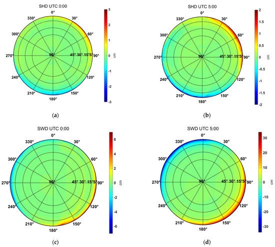
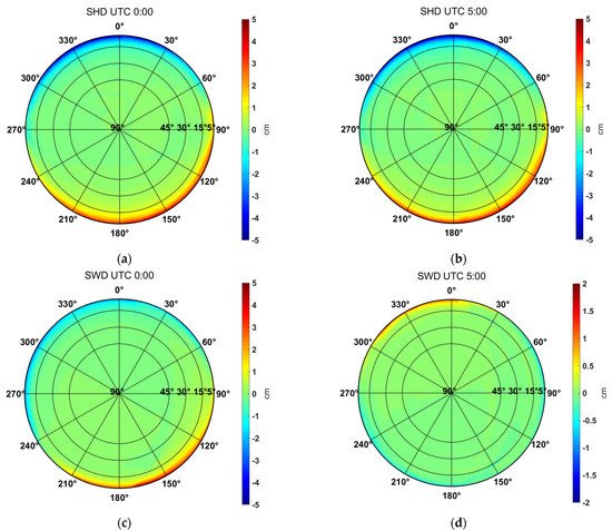
Figure 17. The asymmetry of ray-tracing slant delays calculated by removal of the mean value of each elevation on all azimuths, for the IGS station SHAO located in Shanghai on 21 July 2018 (a) SHDs at 00:00 UTC, (b) SHDs at 05:00 UTC, (c) SWDs at 00:00 UTC, (d) SWDs at 05:00 UTC. Please note the difference between the bound of the colour bar on the right side of each subfigure.
Figure 28. The asymmetry of ray-tracing slant delays calculated by removal of the mean value of each elevation, for the IGS station SHAO located in Shanghai on 26 December 2018. (a) SHDs at 00:00 UTC, (b) SHDs at 05:00 UTC, (c) SWDs at 00:00 UTC, (d) SWDs at 05:00 UTC. Please note the difference between the bound of the colorbar.
Figure 17d shows much more significant anisotropy (please note the disparity in the bounds of the colour bars) than Figure 17c, which means that there was a quick variation of SWD from 0:00 to 5:00 UTC. This may be due to the fast-changing distribution of humidity, the typical summer weather conditions at Shanghai, where the SHAO station is located.
The situation is a little different on 26 December. As shown in Figure 28, although the elevation-dependent pattern is similar to Figure 27, SHD shows more spatial variability than SWD this time. The SHD range can reach up to ~10 cm at 5° elevation, while the SWD range is no more than several centimeters. This result may be caused by the fact that there is much less water vapor in winter than in summer in Shanghai. However, a comparison between Figure 28c,d shows that the temporal variations of SWD are still more complicated than SHD.
In order to get a more quantitative investigation on the results at low elevations, we summarise the statistical result of slant delays at four specific elevations: 5°, 10°, 15° and 20° in Table 13 and Table 24. There is much in common between the two tables. Firstly, the SHD and SWD and their range and RMS all tend to increase positively as elevation angle decreases. However, the SHD is always 6–15 times as large as the SWD. Secondly, the RMS of SHD and SWD at an elevation above 15° are mainly at the level of several millimetres. Furthermore, the RMS and range at the 5° elevation are always ten times as lager as that at the 20° elevation, both for SHD and SWD. Results above indicate that both the SHD and the SWD may present decametric asymmetry at low elevations.
Table 13. Representative ray-tracing slant delays for SHAO located in Shanghai on 21 July 2018.
| UTC | Elevation Angle |
SHD (m) | SWD (m) | ||||
|---|---|---|---|---|---|---|---|
| Mean | Range | RMS | Mean | Range | RMS | ||
| RMS | |||||||
| Mean | Range | RMS | |||||
| 0:00 | 5° | 23.135 | 0.040 | 0.012 | 3.515 | 0.119 | 0.037 |
2.2. TMF Fitting
The results of the four fitting schemes introduced in Table 1 are listed in Table 35, in which elevations are divided into two bands: low elevation (3°≤θ≤15°) and high elevation (15°<θ<90°). As shown in Table 35, there is no apparent difference for bias and RMS between the two elevation and azimuth angle selection strategies (1 vs. 2, or 3 vs. 4). However, the horizontal resolution of ERA5 has a significant impact on the results. The RMS of the fitted SWDs based on ERA5 with 1° × 1° horizontal resolution is four and 7~9 times larger than that of the 0.25° × 0.25°, at low and high elevation angle bands, respectively. Results for SHD are similar but a little better. Hence, we use Scheme 2 in Table 1 (ERA5 with a horizontal resolution of 0.25° × 0.25°, at 18 selected elevations and 24 azimuths) to implement ray-tracing in the following research, which aims to keep a balance between the computational accuracy and the efficiency.
Table 35. Statistic result of TMF-derived slant delays, which are the product of the TMF and the ray-traced zenith delays. The meaning of the postfix numbers is listed in Table 2.
| Elevation Angle |
ΔSHD (cm) | ||||||||||||||||||||
|---|---|---|---|---|---|---|---|---|---|---|---|---|---|---|---|---|---|---|---|---|---|
| bias1 | RMS1 | bias2 | RMS2 | bias3 | RMS3 | bias4 | RMS4 | ||||||||||||||
| 5° | 23.525 | 0.100 | 0.034 | 1.632 | 0.075 | 0.026 | |||||||||||||||
| 0:00 | 10° | 12.896 | 0.035 | 0.012 | |||||||||||||||||
| 3°–15° | 0.0 | 0.3 | 0.0 | 0.3 | −0.3 | 0.7 | −0.3 | 0.7 | 10° | 12.706 | 0.015 | 0.004 | 1.850 | 0.029 | 0.007 | ||||||
| 0.858 | 0.024 | 0.008 | |||||||||||||||||||
| 15°–89° | 0.0 | 0.0 | 0.0 | 0.1 | −0.2 | 0.3 | −0.2 | 0.3 | 15° | 8.703 | 0.007 | 0.002 | 1.255 | 0.018 | 0.004 | ||||||
| 15° | 8.828 | 0.017 | 0.006 | 0.581 | 0.012 | 0.004 | 20° | 6.636 | 0.004 | 0.001 | 0.953 | ||||||||||
| 20° | 6.730 | 0.010 | 0.003 | 0.440 | 0.007 | ||||||||||||||||
| Elevation Angle |
ΔSWD (cm) | 0.012 | 0.002 | ||||||||||||||||||
| bias1 | 0.003 | ||||||||||||||||||||
| RMS1 | bias2 | RMS2 | bias3 | RMS3 | bias4 | RMS4 | 5:00 | 5° | 23.102 | 0.039 | 0.011 | 3.894 | 0.678 | 5° | 23.492 | 0.100 | 0.035 | 1.540 | 0.022 | 0.007 | |
| 3°–15° | 0.0 | 1.9 | 0.0 | 2.0 | 0.0 | 8.00.245 | |||||||||||||||
| 0.0 | 7.9 | 10° | 12.689 | 0.015 | 0.004 | 2.078 | 5:00 | 10° | 12.876 | 0.0360.245 | 0.080 | ||||||||||
| 0.012 | 0.806 | 0.005 | 0.001 | ||||||||||||||||||
| 15°–89° | 0.0 | 0.3 | 0.1 | 0.4 | 0.4 | 2.8 | 0.3 | 2.8 | 15° | 8.691 | 0.007 | 0.002 | 1.410 | 0.118 | 0.037 | ||||||
| 20° | 6.627 | 0.004 | 0.001 | 1.071 | 0.066 | 0.021 | |||||||||||||||
Table 24. Representative ray-tracing slant delays for SHAO located in Shanghai on 26 December 2018.
| UTC | Elevation Angle |
SHD (m) | SWD (m) | ||||
|---|---|---|---|---|---|---|---|
| Mean | Range | ||||||
| 15° | |||||||
| 8.814 | |||||||
| 0.019 | 0.006 | 0.545 | 0.003 | 0.001 | |||
| 20° | 6.719 | 0.011 | 0.003 | 0.414 | 0.002 | 0.000 | |
2.3. TMF Performance
The MF-derived slant delays are the production of the mapping factors and the ray-traced zenith delay. The discrepancy compared with the ray-traced slant delays can directly reflect the accuracy of a mapping function.
Figure 39 shows the RMS scatters of the discrepancies between MF-derived and ray-traced delays at the 5° elevation angle for the 12 globally distributed IGS stations listed in Table 1, at 96 epochs on four days (doy: 74, 202, 246, and 360) in 2018. Since each station’s computation is independent of each other, such a graph would be an excellent way to reflect the global applicability of a mapping function. As shown in Figure 39, the TMFabc performs the best globally, with RMS of almost the same level for each station. Notably, the station FAIR and YAKT have the highest accuracy of wet delays. This may be due to the cold and dry weather on high latitudes in the northern hemisphere.
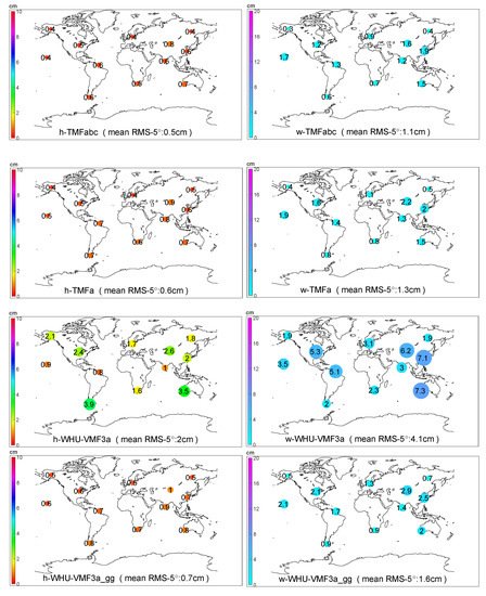
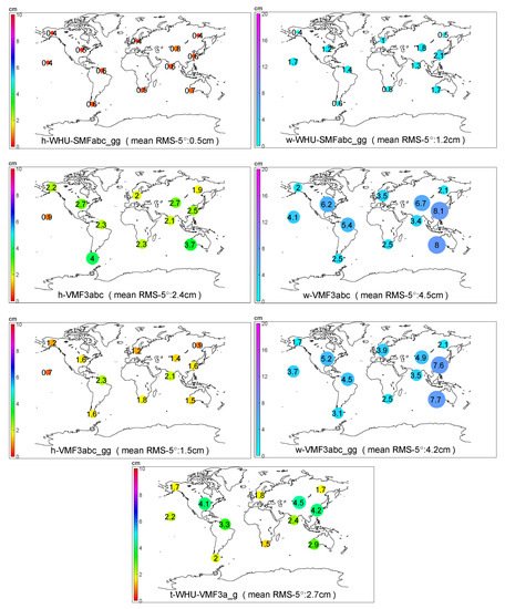
Figure 39. The RMS of various mapping functions at the 5° elevation angle without or with gradients estimation for the 12 IGS stations on doy 74, 202, 246, and 360 in 2018. The size and the color of a circle denote the RMS5° value of the station, of which digit is also marked inside the circle.
In contrast, there are much more variations with the symmetric mapping functions based on the VMF3 concept (WHU-VMF3a, WHU-VMF3a_gg, and WHU-VMF3a_g), especially for the wet delays. However, comparing WHU-VMF3a_gg with WHU-VMF3a shows that the estimation of gradients improves the result dramatically, although not as good as that of TMFs.
The performances of the original VMF3 (VMF3abc and VMF3abc_gg) are the worst but not surprising since the resolution of the NWM used by us (0.25° × 0.25°, 137 model levels, 1 h) is superior to that of VMF3 (1° × 1°, 25 pressure levels, 6 h [40]). VMF3abc_gg improves accuracy mainly on hydrostatic delays but very slightly on wet delays. We can conclude that the resolution of the NWM limits the accuracy of VMF3-derived wet gradients.
TMFabc performs the best among all hydrostatic mapping functions, with the minimal RMSall (RMS for all elevation angles) and the minimal RMS5° (RMS for the 5° elevation angle). Compared with WHU-VMF3a, TMFabc improves the RMSall and the RMS5° by 68% and 74%, respectively. By the extra estimation of hydrostatic gradients, WHU-VMF3a_gg improves these by 62% and 65%, respectively. The accuracy of WHU-SMFabc_gg is only slightly lower than TMFabc. For VMF3, with gradients, the RMSall and the RMS5° can be improved by 35% and 39%, respectively. However, it seems that there are some slight systematic errors between the VMF3-derived and the WHURT-derived hydrostatic slant delays, which would be mainly due to the difference in the NWMs. By adopting the b and c coefficients of VMF3, TMFa can achieve higher accuracy than WHU-VMF3a_gg, with less computational cost than TMFabc, which could be meaningful for large-scale computing.
All MF-derived wet delays’ biases are closer to zero than the hydrostatic ones, but mostly with larger RMSs. TMFabc is still the most accurate, followed by the WHU-SMFabc_gg and TMFa. There is no significant difference between TMFabc and WHU-SMFabc_gg for most stations at most epochs, except for some particular conditions. Figure 410 shows this exemplarily for IGS station SHAO on the doy 202, 2018, when typhoon “Ampil” passed Shanghai. During 3:00–5:00 and 18:00–20:00 UTC, there are apparent improvements for TMFabc against WHU-SMF3abc_gg. WHU-VMF3a_gg improves the RMSall and the RMS5° of WHU-VMF3a by 59% and 62%, respectively.
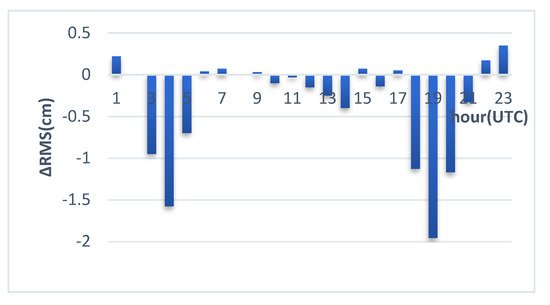
Figure 410. The difference of RMS5° computed by w-TMFabc minus w-WHU-SMFabc_gg for station SHAO (Shanghai, China) for doy 202, 2018.
Figure 511 shows the RMS scatters of all kinds of MF-derived total delays at the 5° elevation angle, which are calculated by rmstotal=rms2h+rms2w−−−−−−−−−−−√, where rmsh, and rmsw are the RMS5° of the hydrostatic and wet MF-derived delays respectively. TMFabc performs the best. The improvement percentage of TMFabc against WHU-VMF3a, WHU-VMF3a_g, and WHU-VMF3a_gg can reach up to 73%, 54%, and 29%, respectively. Even by directly adopting the two coefficients b and c of VMF3 instead of estimating them, TMFa can still improve WHU-VMF3a, WHU-VMF3a_g WHU-VMF3a_gg by 68%, 47%, and 18%, respectively. It is worth noting that the improvement percentage of WHU-VMF3a_gg against WHU-VMF3a_g is 35%, which indicates that a separate estimation of the hydrostatic and wet gradients is preferable to a coarse estimation of the total gradients. Compared with WHU-VMF3a, the reduced RMS5° ratio between WHU-VMF3a_gg and TMFabc is 2.8/3.3, which is close to the value found by Landskron, et al. [46] that two-thirds of the azimuthal asymmetry can be described by the first-order gradients based on the VMF3 mapping function.
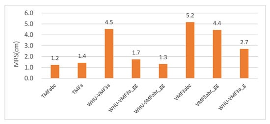
Figure 511. The RMS scatters of MF-derived total delays at the 5° elevation angle (units: cm).
3. Discussion
Investigation of 360-degree ray-traced delays based on NWM revealed that both the SHD and SWD show azimuthal asymmetry, reaching up to decimeter level at low elevation angles below 15°. When a symmetric mapping function is used, the accuracy would not be as bad as expected, since the cutoff elevation angle is always set to 10° or 15° for most geodetic applications, which are typically based on double-differenced solutions. However, significant correlations between troposphere zenith delay parameters, station height, and receiver clock parameters are found [48]. The situation may be considerably improved by lowering the elevation cutoff angle. According to the rule of thumb, the delay path error at a 5° elevation will map to the station height at a ratio of 1/3 [34][36][34,36]. Therefore, it is essential to model variations of the slant delays on the elevation and the azimuth.
The gradient parameters have been used as a supplement for a symmetric mapping function to model the azimuthal asymmetry for decades. However, in former GNSS studies [43][44][45][51][43,44,45,51], only the total gradients can be estimated, due to the difficulty of distinguishing the hydrostatic and wet gradient mapping functions. The WHU-VMF3a_g can be deemed a simulation for such tropospheric delay strategy, of which accuracy is not as good as that of separate estimation of hydrostatic and wet gradients (WHU-VMF3a_gg). In contrast, TMF can achieve better accuracy than a VMF3-like symmetric mapping function enhanced by estimation of respective gradients, of which coefficients b and c are not estimated but obtained from climatology data, and a is determined at a single elevation angle. The result of SMFabc_gg indicates that: (1) If a symmetric mapping function is not accurate enough, it would be difficult to precisely model the anisotropy part of the tropospheric delays by gradients. Therefore, estimating coefficients by least-squares on sufficient widespread elevation angles is necessary. (2) Assuming a proper mapping function is applied, gradients can describe the bulk of the tilting troposphere in most situations. However, there could still be some non-negligible high-order residuals [46], especially under some particular conditions such as severe weather scenarios [62][76].
The assumption of a tilted troposphere can explain most of the actual distribution of the Earth’s troposphere. However, the tropospheric delay error of TMF is about ±1.2 cm at the 5° elevation angle, corresponding to a station height error of ±4 mm. A tilted troposphere may not fully explain the variability of the tropospheric delays, which is also affected by other factors, such as the highly variable water vapor. Therefore, further study should be investigated on how to model the residual delays more precisely based on TMF, if higher accuracy is required. Besides, various NWMs featuring high spatio-temporal resolution produced by different agencies could be utilized together to validate each other and achieve a more robust mapping function.
4. Conclusions
In this research, ERA5 data retrieved from ECMWF with the highest spatial-temporal resolution was applied to compute the tropospheric slant delays by the ray-tracing method. It is found that azimuthal variation of tropospheric delay at low elevation angles can reach up to several decimeters. Traditional three order continued fraction mapping functions have been developed based on the assumption of atmospheric spherical symmetry, in which the azimuthal variation of tropospheric delays is neglected. To overcome shortcomings caused by such mapping functions, TMF is built by tilting the zenith direction of the mapping function, of which coefficients were fitted by Levenberg–Marquardt nonlinear least square method. We found that the horizontal resolution of NWM has a significant impact on mapping functions. However, it is not necessary to choose all elevations and azimuths. Fitting at 18 selected elevations and 24 azimuths are proved to be enough to produce comparable results with complete sampling.
The performances of several mapping functions based on the TMF and VMF3 concept were assessed quantitatively by using the ray-traced slant delays as reference values. Results show that TMF can improve 54% against the VMF3-like symmetric mapping function enhanced by estimating total gradients (WHU-VMF3a_g). According to the rule of thumb, a similar improvement in height parameter estimation is expected in GNSS analysis, which needs to be verified in our further study. A global grid-wise TMF can be developed for an arbitrary station’s interpolation. To balance the accuracy and the computational cost, TMFa may be a good choice. Moreover, it would be necessary for the real-time application to derive TMF based on high-quality operational or forecast versions of NWM, including in-situ meteorological observations if possible.