Rendena is a dual-purpose cattle breed indigenous to the North-East of Italy. This breed is included within the “European Federation of Cattle Breeds of the Alpine System” (FERBA), an organization whose main purpose consists in the preservation and promotion of local cattle breeds of the alpine system (http://www.ferba.info, accessed on 20 April 2021). As is the case with many indigenous breeds, a greater genetic diversity than specialized and cosmopolitan breeds is expected also for the Rendena [1]. This remarkable biodiversity is of great ecological importance and can be a beneficial factor for the survival of the local population. Moreover, traditional breeds such as Rendena provide additional benefits to the local human population such as economic advantages, ecosystem services, and also cultural benefits, such as preservation of cultural heritage and tradition of a specific area [1]. Rendena cattle also shows excellent values for traits concerning fertility and longevity, maintains a median milk production (5000 kg per lactation), and possesses a fairly good beef conformation [2]. Rendena cows are selected for both milk and meat, but with more emphasis on dairy production in the selection index [3], with dairy accounting for 65% and beef traits for 35% [4]. Although beef attitude plays a less important role than milk in the selection index, an increase in the accuracy of the selection for this feature over time could prevent its detriment due to the antagonism with milk production [3]. Estimations of breeding values (EBVs) have until now mostly taken place using classical animal model analysis in Rendena through best linear unbiased predictor (BLUP; [3]) for traits related to milk, meat production, and linear type traits. However, several studies have shown how the use of genomic data can lead to an increase in prediction accuracy compared to using only pedigree information [5].

For a long time, two major limitations to the genomic selection approach on small populations such as Rendena have been the prohibitive cost of genotyping a sufficient number of single nucleotide polymorphisms (SNPs) per individual and the equations for EBVs’ estimation, which were based on a multistep approach [6]. In fact, the drawback of the multistep approach in small populations is the scarce number of genotyped animals with a phenotype to be used as the reference population to ensure a good accuracy of prediction [6]. This is even more noticeable when sex-limited traits are considered [7]. To overcome this problem, methods such as the use of de-regressed proof ^[8][9][8,9] have been developed to allow the inclusion of animals whose only genotype is known, using progeny yield deviation adjusted for mates as a pseudo-phenotype. However, this method presented some biases and lower accuracy whenever animals have few progenies with the phenotype ^[10][11][10,11].

However, in the last few years, both limitations preventing the use of the genomic selection approach in small breeds with limited diffusion such as Rendena have subsided. Firstly, the constant decline in prices of SNP platforms has allowed genomic selection to become much more cost-efficient. Secondly, equations such as the single-step genomic best linear unbiased prediction (ssGBLUP) have been developed and found to be suitable even in small-breed contexts [12]. The ssGBLUP simultaneously evaluates genotyped and non-genotyped animals by substituting the pedigree-based relationship matrix (A) present on BLUP, with a relationship matrix that combines pedigree and genomic information, usually called H [13]. Single-step GBLUP represents a simple alternative to de-regressed proofs. Moreover, ssGBLUP offers the advantage of avoiding double counting contributions, and it implicitly limits the bias of preselection for genotyped animals without the phenotype ^[14][15][16][14,15,16]. Several studies have shown that ssGBLUP outperformed other methods in different livestock species in the context of genomic selection [17]. On the other hand, ssGBLUP might have its own drawback: the genomic relationship matrix (G) included in a single step assumes that all SNPs explain the same amount of variance [18]. This may be a limit in the presence of traits influenced by many quantitative traits loci (QTL), such as some beef-related traits such as carcass weight and daily gain ^[19][20][19,20]. Indeed, some studies reported that SNP regression equations, in which prior assumption of SNPs’ effect and variance are modeled with different a priori assumptions, outperformed the prediction of ssGBLUP [21]. On this point, Zhang et al. [22] proposed to “relax” the assumption of the G matrix in which all SNPs equally contribute to the genomic variance of the traits by adding specific SNPs weights. These methods are called weighted single-step GBLUP (WssGBLUP), and in a recent study, it has been shown to be effective by increasing the accuracy with respect to ssGBLUP for phenotypes such as those related to the beef attitude [23].

2. Variance Components

Heritability (h²) and genetic and residual correlations estimated using PBLUP are reported in Table 2. All traits presented a medium to high heritability. EUROP was the trait with lowest heritability, 0.304, while ADG and DP showed an h² of 0.335 and 0.392, respectively. In addition, all traits’ pairs, as expected, presented medium to high genetic and residual correlations. ADG presented a medium-positive genetic correlation with the other two traits (0.38 on average), while DP and EUROP were strongly correlated (0.981) to be considered a unique trait.

Table 12. Mean of genetic (upper diagonal) and residual (lower diagonal) correlations and heritability (diagonal) between traits in the Rendena population, estimated with PBLUP. Numbers in parenthesis are the lower and the upper 95% highest posterior density.

ADG	EUROP	DP
ADG	0.335 (0.204 ± 0.335)	0.364 (0.100 ± 0.597)	0.398 (0.148 ± 0.6315)
EUROP	0.572 (0.660 ± 0.742)	0.304 (0.174 ± 0.446)	0.981 (0.962 ± 0.997)
DP	0.613 (0.517 ± 0.702)	0.792 (0.753 ± 0.836)	0.392 (0.248 ± 0.541)

ADG = Average daily gain, EUROP = and in vivo fleshiness score CY, DP = in vivo estimate of dressing percentage.

Table 3 reported estimated heritability and genetic and residual correlations using ssGBLUP. In this case, both h² and correlations had similar results to those estimated with the PBLUP. For what concerns h², ADG decreased by about 0.02, while EUROP increased by about 0.04 in ssGBLUP as compared to PBLUP. On the other hand, DP remained basically unchanged comparing the two approaches. Correlations presented almost the same values in both analyses, with the only exceptions of the genetic and residual correlations between ADG and EUROP that resulted in an increase in ssGBLUP of about 0.02 and 0.08, respectively.

Table 23. Mean of genetic (upper diagonal) and residual (lower diagonal) correlation and heritability (diagonal) between traits in Rendena population, estimated with ssGBLUP. Numbers in parenthesis are the lower and the upper 95% highest posterior density.

ADG	EUROP	DP
ADG	0.313 (0.223 ± 0.489)	0.385 (0.153 ± 0.597)	0.392 (0.160 ± 0.622)
EUROP	0.651 (0.651 ± 0.718)	0.345 (0.216 ± 0.487)	0.985 (0.961 ± 0.999)
CY	0.616 (0.530 ± 0.671)	0.790 (0.753 ± 0.826)	0.396 (0.250 ± 0.530)

ADG = Average daily gain, EUROP = and in vivo fleshiness score CY, DP = in vivo estimate of dressing percentage.

3. Weighting Strategies

Figure 12 shows how different values of CT and the limitation of SNPs’ variance can affect genomic prediction.

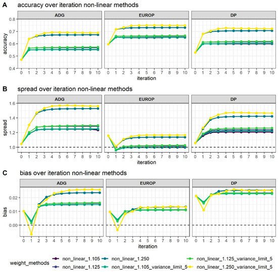
Figure 12. Accuracy (A), dispersion (B), and bias corrected by genetic standard deviations (C) of breeding value estimated using different weighting strategies along the 10 iterations process of the algorithm used in WssGBLUP. The dotted line in Graphs B and C represents the expected value.

As expected, higher accuracy (Figure 2A) was reached in the WssGBLUP analyses with the increase of the number of iterations, although in most cases, the asymptote was reached at the second iteration, with the only exception of the CT 1.25 with the limit of maximum variance established at 5, which reached the maximum accuracy after 3–4 iterations. Variance limits did not affect accuracy using a CT of 1.105 or 1.125.

Bias (Figure 12C) followed the same trends in all phenotypes; at first, iteration bias was even lower than with ssGBLUP, but when iterations increased, bias rapidly increased. ADG presented higher biases, even if the difference in magnitude was considered by standardizing values obtained. Even dispersion (spread; Figure 12B) followed the same trends as accuracy with an increase after 2/4 iterations depending mainly on the value attributed to CT. For all traits, as the interactions increased, dispersion departed from the expected value of 1, although for EUROP, the use of CT at 1.125 was maintained steadily close to 1.

In general, higher CT values (that is, greater departures from normality) presented better accuracy but more under-dispersion and biases. When CT changed from 1.105 to 1.125, accuracy increased by 2% in all phenotypes, and a substantial increase in accuracy was observed, moving to a CT value of 1.250 (+20% on average). When the threshold for maximum SNPs variance was raised up to 5, accuracy increased slightly, especially from the third to tenth iteration.

Figure 23, Figure 34 and Figure 45 show the percentage of variance explained by a sliding window of 20 non-overlapping SNPs. These plots show how the different values of CT and limit influenced the shrinkage SNPs. Furthermore, observing the peaks in the Manhattan plots, it can be seen how these traits are potentially controlled by few QTLs. The high peak found on chromosome 22 for EUROP and DP can explain why these traits are highly genetically correlated.

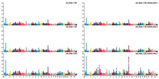
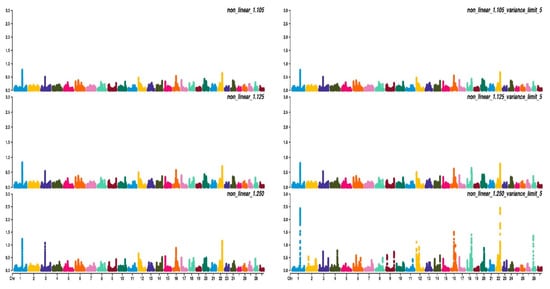
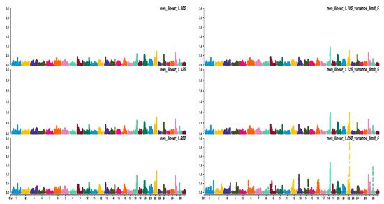
Figure 23. Manhattan plots for average daily gain (ADG) using different WssGBLUP strategies in iterations equal to 10; y-axes represent the percentage explained by each SNP. Variance explained was calculated with a sliding window approach.

Figure 34. Manhattan plots for fleshiness score (EUROP) using different WssGBLUP strategies in iteration equal to 10; y-axes represent the percentage explained by each SNP. Variance explained was calculated with the sliding window approach.

Figure 45. Manhattan plots for dressing percentage (DP) using different WssGBLUP strategies in iterations equal to 10; y-axes represent the percentage explained by each SNP. Variance explained was calculated with the sliding window approach.