1. Introduction

Coastal structures, such as seawalls and breakwaters, provide protection from the effects of the sea and create the conditions for economic growth in coastal environments. These maritime structures also protect ports and coasts against sea dynamics, and their function will be even more important in the upcoming years due to sea level rise and coastal regression as a result of global warming ^[1]. Regarding maritime structures and nearby environments, the effects of sea level rise will include: increasing levels of sediment transport and erosion, higher impacts of wave energy on structures, the loss of stability, and increasing overtopping events ^[2]. On the other hand, increased maritime traffic and human activities along coasts make the proper study and modelling of wave–structure–seabed interactions indispensable in achieving a balance between human intervention, costs, and environmental impacts.

The design of maritime structures must satisfy the project requirements against wind-wave actions [3,4]^[3][4] during the structure service life. The uncertainty in maritime structure design increases when its environment is also considered, especially the seabed, which is the foundation of the breakwater. Some structure failure examples due to seabed failure have been reported in the literature [5,6]^[5][6]. In fact, historical studies reveal that scour is one of the main reasons behind the failure of coastal maritime structures, such as seawalls, groynes, breakwaters, revetments, and artificial reefs [7,8]^[7][8].

Sediment transport has been the subject of extensive research over recent decades, particularly wave–structure interactions and, more importantly, their effects on the seabed. It includes mechanical models [9^[9][10],10], analytical solutions of wave–structure–seabed interactions [11^[11][12][13],12,13], and their verification with numerical models and experimental tests. Physical models of laboratory experiments face very serious problems with sediment and wave scale, even when the prototype with the Froude scale in a laboratory is well achieved. Despite the problems and issues that still arise in the experimental testing of the seabed response, several studies have investigated sediment transport and the scour around maritime structures.

Numerical models appear to be a valuable tool in designing protective structures and performing parametric studies because of the prohibitive cost of field and laboratory experiments. Numerical modelling requires an integral method that incorporates the processes and effects (displacement, stresses, pressures, etc.) between the wave, seabed, and maritime structure. Few numerical models address sediment transport at scales of practical engineering interest or consider multiphase effects and coupled interaction responses. This is usually attributed to either the lack of understanding of the underlying physics or to the fact that multi-scale physics become too computationally and time expensive when dealing with problems at a practical scale.

Several review papers on sediment transport and seabed response have been published; the topics include: (i) analytical formulas for calculating the scour depth around piers [23^[14][15],24], (ii) analytical and experimental studies of scour around coastal structures [25^[16][17],26], and (iii) However, given the great progress made in numerical modelling in the last decade, there is a need to put the most widely used numerical approaches for modelling the wave–structure–seabed interactions into context and focus. For example, for the swash zone, situated at the landward edge of the inundated part of a coastal region, or for numerical simulations of near-shore regions (where the water depth is much smaller than the wavelength, h/L<<1), the use of depth-averaged models that are based on the Shallow Water Equations (SWE) [28]^[18] allow for modelling short wave events and studying the morphological evolution of the coastal zone [29]^[19], and the scour and deposition around structures [30,31]^[20][21]. In the seabed response and sediment transport around maritime structures, the models that are based on RANS equations give an adequate description of the wave–structure interactions, as well as the turbulent flow and bottom boundary layer.

Hence, this paper presents a comprehensive review of the numerical approaches for modelling the seabed response, in particular the scour, around maritime structures that are based on RANS equations for modelling the wave–structure interactions. The review focuses, for the most part, on numerical model papers that were published in the last 10 years and the main keywords used for this review are: scour, sediment transport, numerical modelling, breakwaters, piles, RANS equations, Biot equations, multiphase theory, and fluid–structure–seabed–interactions (FSSI).

Section 2 gathers definitions and physical processes that are involved in the wave–structure interactions that contribute to scour. Section 3 describes the general methodology of each numerical approach. This Section also discusses the applicability, performances, and comparisons between the numerical approaches. Finally, Section 4 presents the closing comments and future scopes of research in this area.

2. Damage to Structures and Coastline: The Role of Scour

This section includes a description of the seabed response, scour, and the consequences on maritime structures and coastlines. In addition, the wave–structure interactions processes that induce sediment transport around structures are discussed.

The presence of the protection structure changes the flow patterns in its immediate vicinity, inducing wave reflection and breaking, turbulence, and liquefaction [34]^[22]. These processes increase the fluid shear stress at the bottom (τf,b) and cause transport when a critical value (τcr,s) is reached. Increased local sediment transport leads to one of the greatest problems for coastal regions and marine structures: scour [35,36]^[23][24]. Scour around coastal structures is the additional erosion that takes place due to hydrodynamic forces acting on the seabed (Figure 1).

Scour has significant impacts on the economic and service life of many coastal structures [21]^[25]. When scour undermines the structure, it cannot support the armour layer of a breakwater, which then slides and loses the fill material. Scour also impacts vertical-front caissons of breakwaters and other gravity structures (Figure 2). More details on scour around such structures can be found in the textbooks of Whitehouse [36]^[24] and Sumer and Fredsoe [34]^[22].

Damage to structures is not the only consequence of seabed scour. In fact, the presence of coastal structures can accelerate the erosion (and deposition), thus degrading coastlines [37,38,39], as shown in Figure 1^[26][27][28]. These examples of structural collapse or a loss of material along the coastline result from both transformation and interaction processes between marine dynamics, especially waves, and the coastal structure.

This process involves an increase in wave height and wave energy, in front of the structure, i.e., greater shear stresses on the seabed and, thus, sediment transport. Wave dissipation: when waves impact a coastal structure, part of its incident wave energy is dissipated by (Figure 3): Among these, wave-breaking on the wall or slope mainly affects sediment transport, which generates turbulence in front of the structure and then mobilizes sediment.(B)Wave diffraction and refraction: when waves interact with an obstacle or coastline, part of the incident energy is concentrated or dispersed in a certain direction, which induces variations in the wave height and flow velocity, causing non-uniform erosion or sediment deposition [45,46]^[29][30]. Furthermore, waves that interact with submerged breakwaters are reduced by a number of energy dissipation mechanisms, including wave breaking and frictional dissipation [47^[31][32],48], which can cause sediment transport around these structures.(C)Turbulent flow around the structure: the flow contraction and velocity field generate turbulence and vortexes around and in front of the structure (Figure 4), which increase the bottom shear stresses (τf,b) and sediment mobilization [34,43]^[22][33].

Wave energy transformation by its interactions with the structure [3,41,42]^[3][34][35]: This process involves an increase in wave height and wave energy, in front of the structure, i.e., greater shear stresses on the seabed and, thus, sediment transport. Wave dissipation: when waves impact a coastal structure, part of its incident wave energy is dissipated by (Figure 3): Among these, wave-breaking on the wall or slope mainly affects sediment transport, which generates turbulence in front of the structure and then mobilizes sediment.

Wave reflection: sediment transport due to wave reflection is perhaps the most commonly cited process in structure–seabed interactions [43]^[33]. The presence of a maritime structure transforms the incident wave energy into reflected energy, which is returned to the sea (Figure 3). This process involves an increase in wave height and wave energy, in front of the structure, i.e., greater shear stresses on the seabed and, thus, sediment transport.

Wave dissipation: when waves impact a coastal structure, part of its incident wave energy is dissipated by (Figure 3): (a) wave-breaking on the slope or wall, (b) turbulent interactions (circulation and friction) with the armour layer, and (c) wave propagation through the porous media of the structure [44]^[36]. Among these, wave-breaking on the wall or slope mainly affects sediment transport, which generates turbulence in front of the structure and then mobilizes sediment.

Wave diffraction and refraction: when waves interact with an obstacle or coastline, part of the incident energy is concentrated or dispersed in a certain direction, which induces variations in the wave height and flow velocity, causing non-uniform erosion or sediment deposition [45,46]^[29][30]. Furthermore, waves that interact with submerged breakwaters are reduced by a number of energy dissipation mechanisms, including wave breaking and frictional dissipation [47,48]^[31][32], which can cause sediment transport around these structures.

Turbulent flow around the structure: the flow contraction and velocity field generate turbulence and vortexes around and in front of the structure (Figure 4), which increase the bottom shear stresses (τf,b) and sediment mobilization [34,43]^[22][33]. Some figures of Higuera et al. [49]^[37] show the increase of turbulence kinetic energy (k=u2+v2+w22) in front of and around a vertical wall and a porous breakwater.

Liquefaction: the pressure differential in the soil may produce the liquefaction of the seabed [13,50,51]^[13][38][39], which leads to the loss of the seabed load-bearing capacity. The liquefaction phenomenon happens when the soil effective stresses are cancelled due to an increase of the pore water pressure. Figure 5 shows the stress field and pore pressure in front of a maritime structure. It can be seen how the effective normal stress (σs′) decreases as the wave-induced pore pressure (ps) increases.

The wave energy transformation by its interactions with a maritime structure. The analysis of the wave energy transformation modes can be achieved by defining a finite control volume (CV) with a unit width and constant depth that includes the structure. The wave energy conservation equation in the control volume is given by FI−FR−FT−D′*=0 [52]^[40], with Fi, i=I, R, and T being the mean energy flux of the incident, reflected, and transmitted wave trains, respectively; and, D′* the mean bulk dissipation.

(a) The flow velocity increases around a composite vertical breakwater; (b) the turbulence kinetic energy Both of the figures are adapted from the numerical simulations to study the interactions between ocean waves and maritime structures performed by Ye et al.

(a) The temporal evolution of the wave induced pore pressure, ps; (b) effective normal stress of the soil in front of a composite vertical breakwater, σs′ (adapted from Ye et al. [53]^[41]).

3. Numerical Modelling of Seabed Response

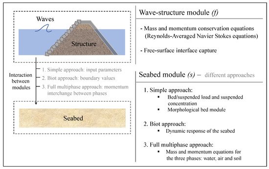
This section presents the governing equations and general methodology of three main Eulerian approaches, in this paper called (i) simple approach (Section 3.1), (ii) Biot approach (Section 3.2), and (iii) full multiphase approach (Section 3.3), for modelling the sediment transport and, thus, the seabed response around maritime structures. The numerical approaches attempt to capture the processes that are involved in the interactions of waves with the structure and their consequences on the seabed foundation. Figure 6 shows a general outline of the numerical approaches described hereafter, which are based on the Reynolds-Averaged Navier–Stokes (RANS) equations (the mass and momentum conservation equations) for the wave–structure interactions and mainly differ in the way that they model the seabed behaviour. This section also shows the applicability and summarizes the performance and parameters used for each numerical methods.

The simple approach decomposes the wave–structure–seabed problem into three modules: ( 1) wave propagation and transformation with the structure, (2) bed load and suspended sediment transport, and (3) bed morphological changes. Figure 7 shows a summary diagram of the modules, parameters, and the interactions between modules. A detailed description of the modules is given below.

The incompressible Reynolds-Averaged Navier–Sshows a general outokes (RANS) equations are applied as the governing equations of fluid flow. These are time-averaged conservation equations of mass and momentum, which describe the mean flow field, respectively:(1)∂uf,i∂xi=0 Equations (1) and (2) have the following considerations:The resulting flow variables (e.g., uf, pf) describe the mean flow field. is estimated using semi-empine of the numerical models.

The resulting flow variables (e.g., uf, pf) describe the mean flow field. Turbulence effects are introduced via the Reynolds’s stresses in the momentum equation, which must be modelled using a turbulence closure.

The turbulence models are usually based on the Boussinesq’s eddy viscosity hypothesis: νT∂uf,i∂xj+∂uf,j∂xi. The eddy viscosity νT is estimated using semi-empirical models.

The free-surfoace of the waves and flow inside the porous media of the structure should be considered in this module.

Density variations are considered in some instances. In this case, an extra density-weighted averaging step is carried out, which results in the Favre-Averaged Navier–Stokes equations (FANS).

This review paper does not focus on the different turs describulence models and Blondeaux et al. [55] provides a detailed description of td he flow–structure by comparing various turbulence models. However, it should be noted that, in the study of wave–structure–seabed interactions, the most appropriate turbulence model should provide an accurate description of (i) the flow close to the bottom (seabed surface) to obtain a reliable evaluation of the sediments transported by the flow [56] and (ii) the turbulent flow generated by the interaeafter, whictions with the structure. The turbulence models used in the papers cited in this work are summarized in Section 3.1.4, Section 3.2.2, and Section 3.3.2, respectively.

Capturing the free surface is essential for modelling wave motion and wave-are breaking. The Volume Of Fluid (VOF) technique is one of the most common methods to track the free surface location [54,57].sed on This method determines the phase within each cell in the domain by introducing an indicator function, ϕ (ϕ=1 full of water, ϕ=0 full of air, interface 0<ϕ<1), and solves the momentum equation (Equation (2)) for a pseudo fluid whose properties are weighted sums based on ϕ. The distribution of ϕ is determined by solving a simple VOF advection equation:(3)∂ϕ∂t+∂(ϕuf,i)∂xi=0

An alternative interface capturing method is the Level Set Method (LSM) that was proposed by Osher and Sethian [58], in which the interface is implicitly represented by the zero level set of a smooth signed distance function that adopts negative values in a phase, zero in the interphase, and positive values in the other phase. Across this region, a Heaviside function is used to smooth sharp flow variable changes and ensure numerical stability. In comparison with the VOF method, the LSM is more accurate in the capture of high curvature interfaces. However, it is not capable of ensuring mass conservation, which is a major drawback in comparison with the VOF method [59].

If the coastal structure is permeable, i.e., formed by a porous material, then the numerical approach should calculate the flow inside the porous media. In this case, the e RANS equations need an additional volume-based averaging step to account for low porosity materials, n∈ (0.35–0.65) (being n, the porosity of the permeable structure), such as those that are normally found in coastal engineering structures. Hence, RANS equations are integrated into a porous control volume, obtaining the Volumeynolds-Averaged Reynolds-Averaged Navier–Stokes equations (VA(RANS)

Equations (4)–(6) are the mass, momentum, and phase volume fraction conservation equations inside the porous media, respectively. After volume averaging, three new terms appear on the right hand side of Equation (5), which are closure terms to account for the frictional and pressure forces, as well as the added mass of the individual components of the porous media. These three terms are drag forces that characterize the flow through the porous media [61]: the lins (the mass and momenear term (laminar flow), auf,i; the quadratic term (turbulent flow), buf,i|uf,i|; and, the inertial acceleration (unsteady flow) term c∂uf,i∂t. The coefficients a, b, and c depend on the physical properties of the material and control the balance between each of the friction terms [62,63].

Note that, for impermeable structures, a non-slip (uf=0) boundary condition is imposed on the structure surface and the goum conserverning equations in the wave–structure module in the case of RANS en equations.

This module includes the calculation of the bed load and suspended sediment transport. Numerous bed load equations have been developed over the past century, qB. The formulas are often empirical and they are commonly based on excess shear stress, where the shear stress is greater than the critical value for incipient motion (τb,f>τcr,s). Bedload equations can include parameters for the characteristics of the fluid and the seabed, such as bed-forms (flat bed or ripples), slope, and sediment composition with τf,b the bottom shear stress of the fluid (from the wawave–structure module); τcr,s∼d50(ρs−ρf)g, the critical bed shear stress; and, d50 and ρs, the characteristic diameter and density of the sediment, respectively.

Forinteractions the suspended sediment transport, the suspended concentration (cs) is often calculated by the advection–diffusion equation (Equation (8)) [67,68], but other papers use ed mpirical formulas for cs as Ahmad et al. [69], who used the empirical formula of Rouse [70]; and, others used empirical formulas for the total sediment transport load (bed and suspended), such as Tofany et al. Concerning the suspended concentration, the suspended load transport is calculated by:(9)qS=∫zuf,xcsdz

It is based on the sediment local mass balance and it involves a non-linear propagation oy diff the bed-level deformationr in the direction of the sediment transport and the spacial variation of the sediment fluxes between the bed load and suspended load [69]. The equation is defined as:(10)∂hs∂t+11−ns∂qt,i∂xi+E−D=0 where qt =qB+qS is the total load transport; ns is the seabed porositway; and, the term (E−D) defines the net sediment movement of the suspended load [74]. Here, E and D are thathe erosion and deposition rates, whose expressions depend on the settling velocity, ws, and the volumetric reference concentration at the bed (cb).

Ththey mode simple approach is used, in particular, for estimating the scour around structures with low weight-structure load on the seabed, such as submarine pipelines. Furthermore, Chen [77] developed the seabed beha Lagrangian–Eulerian model based on the two-dimensional (2D) Navier–Stokes equations for the wave field, and a bed load sediment transport and morphological model to simulate the scouring process in front of a vertical-wall. [78] calculated the 2D flow and sediment transport in front of a breakwater, coupling a morphological model with Navier–Stokes equations. our. They used a 2D RANS-VOF model with additional bottom shear stresses in the momentum equations, coupled with turbulence closure, sediment transport load, and morphological model.

In s section alsome studies, the seabed deformation is accounted for using an interface tracking method [69,84]. [76] used a mesh deformation technique, howhich might be more accurate, but it is noticeably more expensive from a computational perspective. Seabed deformation (either using an interface tracking method or mesh deformation) allows for two-way coupling between the fluid region and seabed. This is often not the case in other more complex approaches, such as the RANS–Biot combination.

An alternative to the simple method for descrithe applicabing wave-–seabed interactions around marine structures is to combine Biot theory [85] (see Equations (11)–(13)) with the Navier–Stokes (NS) equations for the wave field. This numerical approach studies the wave–structure–seabed interactions with two modules: (1) the wave–structure module, based on RANS or VARANS equations as with the simple approach (see Section 3.1.1), and (2) the seabed module (described below) in which the Biot’s equations govern the dynamic response of the porous seabed under wave loading. Figure 9 presents a summary of the modules that are presented in this numerical approach.

The Biot’s equations are adopted as the governing equations for describing the dynamic response of the isotropic porous seabed under wave loading [85]. This paper provides a brief outline of the Biot’s equations, but further details can be found in Jeng and Ou [86]. (1)The momentum conservation equation for the mixture (fluid and sediment) can be written as: (11)∂σs,i′∂xi+∂τs,ij∂xj+ρgi=ρ∂2xs,i∂t2+ρf∂2wf,i∂t2(2)When considering the flow to be governed by Darcy’s law, the momentum equation of fluid phase is written as: (12)−∂ps∂xi+ρfgi=ρf∂2xs,i∂t2+ρfns∂2wf,i∂t2+ρfgiks∂wf ,i∂t(3)The mass conservation equation for fluid phase can be stated as;

The momentum conservation equation for the mixture (fluid and sediment) can be written as: (11)∂σs,i′∂xi+∂τs,ij∂xj+ρgi=ρ∂2xs,i∂t2+ρf∂2wf,i∂t2

When considering the flow to be governed by Darcy’s law, the momentum equation of fluid phase is written as: (12)−∂ps∂xi+ρfgi=ρf∂2xs,i∂t2+ρfns∂2wf,i∂t2+ρfgiks∂wf,i∂t

The mass conservation equation for fluid phase can be stated as; (13)∂∂t∂xs,i∂xi+∂∂t∂wf,i∂xi=−nsKf∂ps∂t

In these equations, σs′ and τs are the effective normal and shear stresses of the soil, respectively; ps is the wave-induced oscillatory pore pressure; xs=(xs ,x,xs,y,xs,ty and summariz) is the seabed displacement; wf is the averaged (Darcy) fluid velocity; ks and ns are the permeability and porosity of the seabed, respectively; ρ=ρfns+ρs(1−ns) is the total density; and, Kf is the bulk modulus of pore water that is related with the degree of saturation of the seabed, Sr. For this module, there are two considerations to be taken into account: (i) the inertial terms and (ii) the rheological model that relates the stresses and deformation of the seabed under wave action.

Different exs the performance and pressions for the Biot’s equations are implemented, depending on the rate of wave loading (wave period, Tw) and the characteristics of the porous media (permeability, ks) [87,88,89]:Fully dynamic: thramete coupled equations of flow and deformation are formulated to include both acceleration terms: ∂2xs,i∂t2, ∂2wf,i∂t2Partly dynamic, which is also known as u−P dynamic: the coupled equations of flow and deformation are formulated when only considering the acceleration of the seabed, ∂2xs,i∂t2.Quasi-static: both inertial terms are ignored, resulting in quasi-static coupled flow and deformation formulation.

Fully dynamic: ts used for eache coupled equations of flow and deformation are formulated to include both acceleration terms: ∂2xs,i∂t2, ∂2wf,i∂t2

Partly dynamic, which is also known as u−P dynamic: thnume coupled equations of flow and deformation are formulated when only considering the acceleration of the seabed, ∂2xs,i∂t2.

Quasi-static: both inertial terical ms are ignored, resulting in quasi-static coupled flow and deformation formulation.

Tthe response of the wave–seabed interactions can be evaluated by rheological models, which relate the normal and shear stresses, (σs′, τs), and the strain, ϵs=∂xs,i∂xi, of the soil under the cyclic wave actionds. Most of the works analyse the wave–structure interactions on non-cohesive seabeds, i.e., composed by sands and/or gravels. For cohesive seabeds (silts and clays), the lack of laboratory or field tests makes it difficult to calibrate and validate the numerical models. A detailed description of rheological models for cohesive and non-cohesive soils is given in Díaz-Carrasco [90].

Most of the papers study the seabed response that is composed of non-cohesive sediments that behave primarily as elastic materials that, in contact with water, have a pore-elastic (dense seabed) [91,92] or pore-elastoplastic (loose seabed) behaviour [86,93,94,95].

The steps to interact the results of the wave–structure module with the seabed module are the following:1.The wave-induced pressure and bottom shear stresses determined in the wave module are the boundary conditions for the seabed module: ,b=τs at the seabed surface.2.The initial consolidation state of the seabed due to static wave and structure loading has to be determined before the dynamic wave loading is applied in the numerical model. This initial consolidation state of the seabed will be the initial stress state for the dynamic seabed response under wave

The wave-induced pressure and bottom shear stresses determined in the wave module are the boundary conditions for the seabed module: ps=pf and τf ,b=τs at the seabed surface.

The initial consolidation state of the seabed due to static wave and structure loading has to be determined before the dynamic wave loading is applied in the numerical model. This initial consolidation state of the seabed will be the initial stress state for the dynamic seabed response under wave loading.

The seabed’s feedback effect on the wave and structure motions (two-way coupling) is neglected.

Their results focus more on the mechanical behaviour (stress field and pressure) of the bearing seabed under wave loading and its interactions with the structure. [95] used the same approach to study the wave–structure–seabed interactions. [84] developed an open-source numerical toolbox for modelling the porous seabed interactions with waves and structures in the finite-volume-method (FVM)-based OpenFOAM framework. In fact, these works generally study the liquefaction phenomenon that is induced by wave action and how it affects the structure.

Table 2 summarizes the performance and parameters for developing the RANS–Biot approach of the most relevant studies found. Most of these studies consider the effects of wave breaking and wave–structure interactions, for which they use the VARANS equations in combination with the VOF method. Most of these studies use the u−p approximation for the inertial terms in the Biot’s equations, which offers improved results over the quasi-static formulation [88]. Elsafti and Oumeraci [109] observed that this approximation significantly reduces the computational time, and it should be considered whenever pore fluid acceleration is negligible.

The movement of sediments due to the fluid flow is a two-phase phenomenon [110]. The starting point for developing any multiphase model is the local instantaneous formulation, which consists of field equations that are applied to the distinct phases complemented with jump conditions to match the solution at the interface and source terms to account for interactions between phases.

The governing equations for multiphase models are the conservation equations of mass and momentum for each phase. A specific momentum equation is used for the sediment (solid phase). However, specific continuity equations are necessary for each phase since the system now includes three phases. The last two terms in the momentum equations are related to momentum interchanges between the sediment and fluid phases: the first term accounts for the drag force and the second term for turbulent dispersion.

Mass conservation equations: (14)∂cs∂t+∂(csus,i)∂xi=0;Sedimentphase (15)∂(1−cs)ϕ∂t+∂(1−cs)ϕuf, i∂xi=0;Waterphase

Momentum conservation equations: (17)∂ρf(1−cs)uf,i∂t+∂ρf(1−cs)uf,iuf,i∂xi=ρf(1−cs)gi−(1−cs)∂pf∂xi+∂(1−cs)Tf∂xj−csρsuf,i−us,iτp+ρsτp(1−cs)νSc∂cs∂xi;Fluidphase (18)∂ρscsus,i∂t+∂ρscsus,ius,i∂xi=ρscsgi−cs∂pf∂xi−∂csps∂xi+∂csTs∂xj−csρsuf,i−us,iτp+ρsτp(1−cs)νSc∂cs∂xi;Sedimentphase where the sub-indexes f and s refer to the fluid and sediment phases, respectively; ρ is the density; c is the volume concentration of sediment; u is the velocity; ν is the kinematic viscosity; Sc is the Schmidt number; p is the pressure; T represents the viscous and turbulent stress tensor; and, τp=ρsρf−ρs(1−ws)2g is the response time of the particles, with ws being the settling velocity of the sediment. The last two terms in the momentum equations are related to momentum interchanges between the sediment and fluid phases: the first term accounts for the drag force and the second term for turbulent dispersion.

The application of the full multiphase model allows for greater accuracy regarding sediment movement and seabed–wave–structure response. In this case, the seabed region is modelled as a continuous medium, which provides greater detail in the description of pressure, stresses, and interchange terms between phases. For the high sediment concentration region (near the bed), the model requires a very refined mesh, which leads to a higher computational cost. The studies that are based on this approach mainly focus on small-scale problems that are related with the estimation of the sediment transport around small structures, such as monopiles.

Many models have been developed for the two phases, i.e., water-sediment [111,112,113,114,115,116], and few of them include air as a third phase to handle the free surface tracking. These studies mostly differ in the way they treat closure terms for particle stresses, turbulence, and momentum exchanges. [111] show that adding a turbulence modulation term due to particle presence to the k−ϵ model improves the accuracy in the boundary layer. [115] propose the inclusion of extra rheological terms that account for enduring-contact, as well as viscous and interstitial effects, which extend the range of application of their model to higher Reynolds numbers.

Table 3 proposes a summary of the performance and parameters of the most relevant studies using this approach. The multiphase approach requires turbulence modulation due to the presence of sediment particles. Moreover, momentum exchanges between phases are accounted for by using source terms in the momentum equations. As can be seen, the use of a full multiphase approach requires the consideration of several closure terms for the particle stresses, turbulence stresses, and phase interaction mechanisms, most of which are based on empirical equations.

4. Conclusion and Future Prospects

The main objective of this paper is to present a comprehensive review of the numerical approaches for modelling the wave–structure–seabed interactions, while focusing on the seabed response, i.e., scour. This review is intended to complement the review papers on sediment transport and seabed response around maritime structures, which are mainly based on analytical and experimental studies. For this purpose, a literature review of the main and most recent works (over the last 10 years) on numerical modelling was carried out.

In this paper, they are referred to as: (i) simple approach, (ii) Biot approach, and (ii) full multiphase approach. These three approaches are based on Reynolds-Averaged Navier–Stokes equations for the wave–structure module 1.The simple approach considers: (a) the bed load transport with empirical formulas; (b) the suspended concentration with the advection–diffusion equation and suspended load transport; and, (c) The studies that used Biot’s equations for the seabed module focus more on the stress field and pressures, which is, the mechanical behaviour of the seabed.3.The full multiphase approach is the more complex approach and is difficult to implement numerically.

The simple approach considers: (a) the bed load transport with empirical formulas; (b) the suspended concentration with the advection–diffusion equation and suspended load transport; and, (c) The wave module is mainly based on RANS or VARANS equations, depending on whether the structure is permeable or impermeable. The studies that use the simple modelling approach mainly focus on small and low weight-structures to simulate the movement and deformation of the seabed (two-coupled approach). For large structures, such as breakwaters, these studies tend to underestimate the scouring results.

The Biot approach involves the RANS or VARANS equations for the wave module and the Biot’s equations for the seabed module. Biot’s equations are used to obtain the seabed displacement and stresses. The outputs of the wave module are used as boundary conditions for the seabed module. The studies that used Biot’s equations for the seabed module focus more on the stress field and pressures, which is, the mechanical behaviour of the seabed.

The full multiphase approach is the more complex approach and is difficult to implement numerically. It solves each phase (sediment, water, and air) with the Navier–Stokes equations (mass and momentum) at the same time and space. Most of the studies are based on small-scale problems given the very high computational costs that are associated with its use.

This paper describes the general concept and methodology of each numerical approach for modelling wave–structure–seabed interactions. However, there are certain aspects when developing a numerical model that need to be studied in more detail and that were not the focus of this review: (i) the turbulence model that best characterizes the near-bed turbulent flow–structure and the turbulent flow interactions with the structure; (ii) the particle stresses, which is, the rheological models that provides a functional relation between the stresses and strains of the seabed under wave action; and (iii) the optimal boundary and initial conditions for each numerical approach.

References

- Vousdoukas, M.I.; Mentaschi, L.; Voukouvalas, E.; Verlaan, M.; Feyen, L. Extreme sea levels on the rise along Europe’s coasts. Earth’s Future 2017, 5, 304–323.
- Irie, I.; Nadaoka, K. Laboratory reproduction of seabed scour in front of breakwaters. In Coastal Engineering 1984; American Society of Civil Engineers: Reston, VA, USA, 1985; pp. 1715–1731.
- Burcharth, H.; Hughes, S. Shore Protection Manual. Chapter 6: Fundamentals of design; US Army Corps of Engineers: Washington, DC, USA, 2002; Volume 1.
- ROM 1.1-18. Recommendations for Breakwater Construction Projects; Technical Report; Puertos del Estado: Madrid, Spain, 2018.
- Molinero Guillén, P. Large breakwaters in deep water in northern Spain. In Proceedings of the Institution of Civil Engineers—Maritime Engineering; Thomas Telford Ltd.: London, UK, 2008; Volume 161, pp. 175–186.
- Puzrin, A.M.; Alonso, E.E.; Pinyol, N.M. Geomechanics of Failures; Springer Science & Business Media: Berlin, Germany, 2010.
- Hughes, S. Scour and Scour Protection. Ph.D. Thesis, Coastal and Hydraulics Laboratory, US Army Engineer Research and Development Center, Vicksburg, MS, USA, 1993.
- Sumer, B.M. Coastal and offshore scour/erosion issues-recent advances. In Proceedings of the 4th International Conference on Scour and Erosion (ICSE-4), Tokyo, Japan, 5–7 November 2008; pp. 85–94.
- Maa, P.Y.; Mehta, A. Mud erosion by waves: A laboratory study. Cont. Shelf Res. 1987, 7, 1269–1284.
- Foda, M.A.; Hunt, J.R.; Chou, H.T. A nonlinear model for the fluidization of marine mud by waves. J. Geophys. Res. Ocean. 1993, 98, 7039–7047.
- Tsai, Y.; McDougal, W.; Sollitt, C. Response of finite depth seabed to waves and caisson motion. J. Waterw. Port Coast. Ocean Eng. 1990, 116, 1–20.
- Kumagai, T.; Foda, M.A. Analytical model for response of seabed beneath composite breakwater to wave. J. Waterw. Port Coast. Ocean Eng. 2002, 128, 62–71.
- Liao, C.; Tong, D.; Chen, L. Pore pressure distribution and momentary liquefaction in vicinity of impermeable slope-type breakwater head. Appl. Ocean Res. 2018, 78, 290–306.
- Kumar, A.; Kothyari, U.C.; Raju, K.G.R. Flow structure and scour around circular compound bridge piers—A review. J. Hydro-Environ. Res. 2012, 6, 251–265.
- Gazi, A.H.; Afzal, M.S.; Dey, S. Scour around piers under waves: Current status of research and its future prospect. Water 2019, 11, 2212.
- Sumer, B.M.; Whitehouse, R.J.; Tørum, A. Scour around coastal structures: A summary of recent research. Coast. Eng. 2001, 44, 153–190.
- Sumer, B.M. Mathematical modelling of scour: A review. J. Hydraul. Res. 2007, 45, 723–735.
- Vreugdenhil, C.B. Numerical Methods for Shallow-Water Flow; Springer Science & Business Media: Berlin, Germany, 1994; Volume 13.
- Postacchini, M.; Brocchini, M.; Mancinelli, A.; Landon, M. A multi-purpose, intra-wave, shallow water hydro-morphodynamic solver. Adv. Water Resour. 2012, 38, 13–26.
- Postacchini, M.; Russo, A.; Carniel, S.; Brocchini, M. Assessing the hydro-morphodynamic response of a beach protected by detached, impermeable, submerged breakwaters: A numerical approach. J. Coast. Res. 2016, 32, 590–602.
- Son, S.; Lynett, P.; Ayca, A. Modelling scour and deposition in harbours due to complex tsunami-induced currents. Earth Surf. Process. Landf. 2020, 45, 978–998.
- Sumer, B.M.; Fredsoe, J. The mechanics of scour in the marine environment. In Advanced Series on Ocean Engineering: Volume 17; World Scientific: Singapore, 2002.
- Whitehouse, R. Scour at Marine Structures: A Manual for Practical Applications; Thomas Telford: Telford, UK, 1998.
- Whitehouse, R. Scour at Marine Structures. In Proceedings of the Third International Conference on Scour and Erosion, Amsterdam, The Netherlands, 1–3 November 2006.
- Fausset, S. Field and laboratory investigation into scour around breakwaters. Plymouth Stud. Sci. 2017, 10, 195–238.
- Pilkey, O.H.; Wright III, H.L. Seawalls versus beaches. J. Coast. Res. 1988, 4, 41–64.
- Basco, D. Seawall impacts on adjacent beaches: Separating fact from fiction. J. Coast. Res. 2006, 39, 741–744.
- Balaji, R.; Sathish Kumar, S.; Misra, A. Understanding the effects of seawall construction using a combination of analytical modelling and remote sensing techniques: Case study of Fansa, Gujarat, India. Int. J. Ocean Clim. Syst. 2017, 8, 153–160.
- Tang, J.; Lyu, Y.; Shen, Y.; Zhang, M.; Su, M. Numerical study on influences of breakwater layout on coastal waves, wave-induced currents, sediment transport and beach morphological evolution. Ocean Eng. 2017, 141, 375–387.
- Do, J.D.; Jin, J.Y.; Hyun, S.K.; Jeong, W.M.; Chang, Y.S. Numerical investigation of the effect of wave diffraction on beach erosion/accretion at the Gangneung Harbor, Korea. J. Hydro-Environ. Res. 2020, 29, 31–44.
- Batjest, J.A.; Beji, S. Spectral evolution in waves traveling over a shoal. In Proceedings of the Nonlinear Water Waves Workshop, Bristol, UK, 22–25 October 1991; p. 11.
- Ferrante, V.; Vicinanza, D. Spectral analysis of wave transmission behind submerged breakwaters. In Proceedings of the The Sixteenth International Offshore and Polar Engineering Conference, San Francisco, CA, USA, 28 May–2 June 2006.
- Tait, J.F.; Griggs, G.B. Beach Response to the Presence of a Seawall; Comparison of Field Observations; Technical Report; California University of Santa Cruz: Santa Cruz, CA, USA, 1991.
- Baquerizo, A.; Losada, M.; López, M. Fundamentos del movimiento oscilatorio. In Manuales de Ingeniería y Tecnología; Editorial Universidad de Granada: Granada, Spain, 2005.
- Díaz-Carrasco, P.; Moragues, M.V.; Clavero, M.; Losada, M.Á. 2D water-wave interaction with permeable and impermeable slopes: Dimensional analysis and experimental overview. Coast. Eng. 2020, 158, 103682.
- Clavero, M.; Díaz-Carrasco, P.; Losada, M.Á. Bulk Wave Dissipation in the Armor Layer of Slope Rock and Cube Armored Breakwaters. J. Mar. Sci. Eng. 2020, 8, 152.
- Higuera, P.; Lara, J.L.; Losada, I.J. Three-dimensional interaction of waves and porous coastal structures using OpenFOAM®. Part I: Formulation and validation. Coast. Eng. 2014, 83, 243–258.
- McAnally, W.H.; Friedrichs, C.; Hamilton, D.; Hayter, E.; Shrestha, P.; Rodriguez, H.; Sheremet, A.; Teeter, A.; ASCE Task Committee on Management of Fluid Mud. Management of fluid mud in estuaries, bays, and lakes. I: Present state of understanding on character and behavior. J. Hydraul. Eng. 2007, 133, 9–22.
- Chávez, V.; Mendoza, E.; Silva, R.; Silva, A.; Losada, M.A. An experimental method to verify the failure of coastal structures by wave induced liquefaction of clayey soils. Coast. Eng. 2017, 123, 1–10.
- Losada, I.; Patterson, M.D.; Losada, M. Harmonic generation past a submerged porous step. Coast. Eng. 1997, 31, 281–304.
- Ye, J.; Zhang, Y.; Wang, R.; Zhu, C. Nonlinear interaction between wave, breakwater and its loose seabed foundation: A small-scale case. Ocean Eng. 2014, 91, 300–315.