Rain is a natural process that attenuates the propagating signal at microwave and millimeter-wave frequencies. Therefore, it is necessary to mitigate rain attenuation to ensure the quality of microwave and millimeter-wave links. To this end, dynamic attenuation mitigation methods are implemented alongside attenuation prediction models that can predict the projected attenuation of the links. Studies on rain attenuation are used in geographically distributed locations to analyze and develop a rain attenuation model applicable over a wide frequency range, particularly radio frequencies over approximately 30 GHz for 5G and beyond network applications.
- ITU-R model
- rain attenuation
- millimeter-wave
- rain attenuation time series
1. Preliminaries
1.1. Rain Attenuation Factors
It is crucial to find a justification and insightful analysis to determine the variables that influence rain attenuation. Although rain is a crucial factor influencing rain attenuation, the link distance, frequency, and polarization play a significant role in the determination of rain attenuation. A brief review of more parameters for rain attenuation is presented here. In the literature, various researchers have found different rain attenuation factors for either terrestrial or slant links. In this regard, we compiled 17 parameters that can impact rain attenuation for microwave links using artificial or ML-based techniques [1].
1.2. Rainfall Rate Data Collection Procedures
1.2.1. Available Databases
European Center for Medium-Range Weather Forecasts
ECMWF re-analysis-15
1.2.2. Experimental Setup
A simple method of determining the rain rate is to set up an experiment to deploy measuring equipment such as the use of a disdrometer, weather station, and rain gauges that measure the rain rate at lower integration times (⩽1 min intervals), which can be saved in a personal computer with the help of a dedicated data logger [2][3][4][5]. In some cases, the radar information of the rain cell was used to measure the rain rate. The problem with radar-based techniques is that massive investments are required to collect rain rate information if radar systems have not been deployed for other purposes [6][7].
1.2.3. Rain Rate Data Generation: Synthetic Technique and Logged Data
The rain rate time series in a specific area is essential because it is used to calculate the attenuation in a fixed radio transceiver infrastructure [8]. The general procedure for collecting the rain rate time series is to collect the data by employing an experimental setup. Thus, the general approach is time-consuming because a minimum of one year of data should be collected over a particular area. Cost is also associated with this process. In addition to this experimental technique, a synthetic method can be used to calculate the time series using a mathematical approach.
1.2.4. Rain Rate Prediction from Spatial Interpolation Techniques
To accurately determine the rain attenuation, it is necessary to consider the spatial distribution of the rainfall intensity. The rain rate cannot be measured everywhere using the rain rate collector, which significantly reduces the accuracy of the experimental setup. However, an intense spatial resolution rain rate is required for accurate estimation. There exist some synthetic techniques by which the undetermined rain rate can be estimated to solve the problem at a particular location.The inverse distance weighting (IDW) technique as per Equation (1) can be used to determine the rainfall rate at ungauged locations [9][10]:
where N is the number of rain gauges. The rain value
wi
di
wi
1.125∘×1.125∘
The spatial-temporal rainfall distribution mechanisms based on the top-to-bottom data analysis approaches are surveyed in [11]. This survey compared most techniques that predict high-resolution space-time rainfall using remote sensing, conventional spatial interpolation, atmospheric re-analysis of rainfall, and multi-source blending techniques, and discussed issues in integrating various merging algorithms. In the article, it was shown that the maximum spatial resolution is available by the
Global Satellite Mapping of Precipitation Near Real-Time (GSMaP-NRT)
0.01∘
Another technique for generating the rain rate is applying the local rain data to the MultiEXCELL model [12]. This model was used in [13] to generate synthetic rain rates. Transmitting and detecting specific differential phase-shifted signals through a dual-band radar system has been experimented with in [14]. As a result of this experiment, the authors noticed the scattering effects in the detected signals that arise due to the radar signals’ differential reflection. A corrector factor should be used for the reflected and differently reflected signals in order to eliminate the scattering effects. The statistical uncertainties of rainfall are then calculated by considering the propagation of the power-law relations.
 R(Zh,Zdr,Kdp)=9.6046Z0.072hZ−0.017drK0.824dp.
Table 1.
| Ref. | Estimation Techniques |
|---|
Table 3.
| Ref. | EPL or PCF | Parameter Settings | Remarks |
|---|
| [15] | The proposed technique generates rain attenuation time series using storm speeds from 1 to 12 m/s in a two-layered rain structure model. Also, temperature, altitude, and height are used as per the geographic location. | |||||
| [26] | The proposed technique generates rain attenuation time series using storm speeds from 1 to 12 m/s in a two-layered rain structure model. Also, temperature, altitude, and height are used as per the geographic location. | |||||
| 5] | Analyzed millimeter-wave and showed that the ITU-R predicted rainfall rate of region P is up to 0.01% of time (agrees → 99.99% of time and disagrees → 0.01% of time). | |||||
| [2] | r=1/{1+0.03(100P)βl] | r | ||||
| ∘ | ||||||
| m | }⧫ | Method: Practical measurement; Frequency band: 7–38 GHz; Path length: 58 km; and rain rates were collected over 1-min time interval. | The correction factor depends on β; link length; and p% of rain | |||
| [16] | ||||||
| [27] | [11][22] | |||||
| A | ||||||
| [ | This multi-source blending technique to estimate high-resolution space-time rainfall scales to develop and merge remote sensing, conventional spatial interpolation, atmospheric re-analysis of rainfall, and multi-source blending techniques. | |||||
| 31][3 | rad(t)=Arad,d(t | |||||
| ( | t)=a0⋅e2dAG/βa√⋅W(t)+dAG⋅va/βa⋅t1+dAG⋅a0∫t0e2dAG/βa√⋅W(s)+dAG⋅va/βa⋅sds | |||||
| where | ||||||
| a | 0 | |||||
| :0–0.5 dB, | ||||||
| W | (t) | |||||
| : Wiener process, | ||||||
| β | a | |||||
| , | ||||||
| v | a | |||||
| : gamma distribution parameters, | ||||||
| d | AG | |||||
| : Dynamic parameter | ||||||
| β | ||||||
| of the Maseng-Bakken model. | ||||||
| [17] | ||||||
| [28] | [27][38] | |||||
| It proposed an enhanced technique to generate rain attenuation time series where precise rain rates are not available at global scale using ITU-R model. The technique uses mean and standard deviation of rain rate either from NOAA | [18] and ITU-R model [19] and the output of Gaussian noise through a low-pass filter (LPF: | |||||
| It proposed an enhanced technique to generate rain attenuation time series where precise rain rates are not available at global scale using ITU-R model. The technique uses mean and standard deviation of rain rate either from NOAA [29] and ITU-R model [30] and the output of Gaussian noise through a low-pass filter (LPF: | ||||||
| k | /p+β | |||||
| , cut-off frequency f | ||||||
| c | ||||||
| : 0.2 MHz) into a non-linear memoryless device, where | ||||||
| A | offset | |||||
| is the calibration factor, | ||||||
| A | offset:exp(m+σQ−1(P0/100)) | |||||
| and | ||||||
| Q | ||||||
| : zero-mean, unit variance Gaussian probability density function. | ||||||
| It presented gauged-based data re-analysis at a resolution of | \( 0.5{^\circ}×0.5{^\circ} \) 0.5∘×0.5∘. | |||||
| [20] | ||||||
| [31] | [33][43] | |||||
| A | (x0 | |||||
| r | ||||||
| ) | ||||||
| = | ||||||
| = | ||||||
| 1.08 | ||||||
| k | ||||||
| L | ||||||
| A | ||||||
| − | 0.5108 | |||||
| ∫ | LA0RαA(x0+Δx0,ξ)dξ+kB∫LBLARαB(x0,ξ)dξ | |||||
| where | ||||||
| L | A | |||||
| and | ||||||
| L | B | |||||
| are the radio path lengths, | ||||||
| Δ | x0 | |||||
| is the shift due to the presence of layer B, | ||||||
| x | 0=v⋅t | |||||
| , and | ||||||
| v | ||||||
| is the average storm speed (typically 10 m/s). | ||||||
| (7 GHz for 0.01% of the time) | Method: Practical virtual link; Link length: 1–10 km; Time exceedance: 0.01%; Frequency 7 GHz | The reduction function depends only on the total path length. Estimation: Exponential curve fitting | ||||
| [21] | ||||||
| [32] | ||||||
| [34][44] | ||||||
| A | ||||||
| d | eff | |||||
| ( | t0) | |||||
| = | ||||||
| = | ||||||
| 1 | 1+d/d0 | |||||
| 1 | cosθ | |||||
| ⋅ | ||||||
| [ | ∫d0+SAd0kAR(l)αAdl | |||||
| d | ||||||
| + | ∫d0+SA+S | |||||
| Method: Practical setup; Site: S. Paulo, Brazil; Season: Dry season; Frequency: 15 GHz (4 links) and 18 GHz (2 links) with vertical and horizontal polarizations; Path lengths: 7.5–43 km; Duration: 1–2 year | The correction factor depends only on the rain rate exceedance of | p | % of the time. Estimation: exponential curve fitting | |||
| A copula is a multivariate distribution function expressed by marginally uniform random unit interval variables and it can avoid dependence index like in log-normal distribution. The procedure is: | ||||||
| [33] | ||||||
| [35][45] | A copula is a multivariate distribution function expressed by marginally uniform random unit interval variables and it can avoid dependence index like in log-normal distribution. The procedure is: | |||||
| ρ | = | |||||
| r | (R0.01,L) | |||||
| sin | (πτ2)→ | |||||
| zero mean Gaussian random variables correlated matrix→normal CDF→desired random variable→inverse CDF of the desired distribution. | ||||||
| = | L×(−R0.011+ζ(L)×R0.01)▲ | ITU-R database; Site: 8 countries; Path lengths: 1.3–58 km; Frequency: 11.5–39 GHz; Rain rates (0.1%): 18–105mm/h | The PCF depends on rain rate exceedance %p of time and link length. Estimation: curve fitting | |||
| [23] | The procedure is: | |||||
| [34] | The procedure is: | |||||
| [36][46] | ||||||
| R | G=e−β⋅|τ|→[ | |||||
| r | =3.6435Rp− | |||||
| β | EMB,βgamma]→H(z)=1−e−2βTs√1−z−1e−βTs | |||||
| , where | ||||||
| T | s | |||||
| : sampling time, and | ||||||
| β | EMB | |||||
| and | ||||||
| β | gamma | |||||
| are | ||||||
| 12.3 | d−0.95×10⁻⁴ | |||||
| and | ||||||
| 6.9 | d−0.6×10⁻⁴ | |||||
| , respectively. | ||||||
| [24] | The procedure is: | |||||
| [35] | The procedure is: | |||||
| a | k=1N∑N−1j=0Mje−i2πNkj=I(Mj)→ak=hkI(cG)−−−−−−−√×ek→Mj=I−1 | |||||
| [28][39] | In GSMaP-NRT, it analyzed the satellite, microwave-infrared, and near real time weather dataset to compare better predictability presented resolution about 0.01∘×0.01∘. | |||||
| ) | /γRd | Method: Simulation Frequency: 22 and 38 GHz Path lengths: 2, 5, 10 and 20 km | The correction factor only depends on the Arad,d(t), and γR(t). | 0.377 | Method: Practical setup; Link length: 2.29 km; Rain Gauge: Tipping rain bucket (0.254 mm accuracy); Frequency: 28.75 GHz | The correction factor depends only on the rain rate exceedance of the %p of the time. Estimation: curve fitting. |
| ( | ak),[hk=0.5] | |||||
| , where | ||||||
| M | ||||||
| [32][42] | ||||||
| [37][47] | r(R0.01,d)=d/[ | |||||
| ( | t) | |||||
| : Gaussian process, | ||||||
| ℑ | ||||||
| and | ||||||
| I | −1 | |||||
| are direct and inverse Fourier transforms, respectively. | ||||||
| r | =11+L2636R(P)−6.2 | Method: Practical measurement Rain rate: 5-min point at 11 GHz frequency; 42.5 km long radio link with R>10mm/h | The correction factor depends on the radio link length and rain rate. | [29][40] | ||
| B | d0+SAkB3.134αBR(l)αBdl] | |||||
| , where | ||||||
| θ | ||||||
| :link elevation angle, ( | ||||||
| α | A | |||||
| , | ||||||
| k | A | |||||
| ), ( | ||||||
| α | B | |||||
| , | ||||||
| k | B | |||||
| ): power-law coefficients that converts the rain rate into specific attenuation for layers A and B, respectively, and | ||||||
| R | ||||||
| : rain rate along the link. | ||||||
| ECMWF: | \( 1.125{^\circ}×1.125{^\circ} \) 1.125∘×1.125 | |||||
| [22] | ||||||
| [30][41] | It proposed the spatial and the temporal correlation functions to determine rainfall rate. | 1+{d/2.6379R0.010.21}] | Practical setup; Link length: unavailable; Rain Gauge: Tipping, Frequency: 15 GHz, Availability: 99.95%; Duration: 4 years; Rain rate: R (0.1 to 0.001) | The correction factor depends only on the rain rate exceedance of the %p of the time and LOS link length. Estimation: exponential curve fitting | ||
| [25] | Compute the stochastic differential equation: | |||||
| [36] | Compute the stochastic differential equation: | |||||
| [38][48] | ||||||
| d | A(t | |||||
| r | = | |||||
| ) | ||||||
| 1.303 | ||||||
| = | ||||||
| ς | 1+L | |||||
| μ | 4da(μ2λA(t)−A2(t)+μ2).dt+daμ3λ−−−−√A(t)dW(t) | |||||
| , where | ||||||
| d | a=2βaS2aλμ3 | |||||
| , where | ||||||
| μ | ||||||
| and | ||||||
| γ | ||||||
| are found by fitting to experimental first order statistics of rain attenuation, | ||||||
| β | a | |||||
| and | ||||||
| S | a | |||||
| are the parameters of the diffusion coefficient of the M-B model. | ||||||
| D | ♣ | Model: empirical model, based on the point of inflexion (POI) | The correction factor depends only on the slant path length and the rain cell diameter. | |||
| [26] | Compute: | |||||
| [37] | ||||||
| [39][49] | Compute: | |||||
| P | (ti)=1−P0, | |||||
| r | =A/(kRαTXLslant) | |||||
| i | →zi=Tz(ri)→findMz(d)→GaussianPDF→ρj(τ)→Hi(z) | |||||
| , where | ||||||
| P | 0,i | |||||
| is the possibility of rain in the | ||||||
| i | ||||||
| th station, | ||||||
| r | i | |||||
| represents a nonlinear transformation | ||||||
| T | z | |||||
| , and | ||||||
| ρ | j | |||||
| is the temporal autocorrelation function of rain attenuation for | ||||||
| i | ||||||
| th link. |
Table 2.
| Method: MultiEXCELL rain simulation. Calculation: rain attenuation is calculated via the numerical approach. Rain field size: 1 km × 1 km to 250 km × 250 km | |||
| The correction factor depends on calculated attenuation, specific attenuation conversion coefficients, ‘measured’ rain rate at the transmitter end, and the LOS link length. | |||
| [ | |||
| 40 | |||
| ] | |||
| [ | |||
| 50] | r=1[0.477L0.633R0.073α0.01%f0.123−10.579(1−e−0.024L)] | (1) Can be used worldwide; (2) frequency band: 5–100 GHz; (3) Maximum path length is 60 km | The correction factor depends on the frequency (GHz), specific attenuation coefficient (α), and link length (L). |
| [41][51] | r=⎧⎩⎨⎪⎪Necosθ(hR−hStanθ)Necosθ(10.056+0.012R)R<R0R≥R0 | The number of effective cells (Ne) is calculated after analyzing ITU-R DBSG3 database. | To define the rain cell, it needs to know the cell (R0) boundary rain rate. |
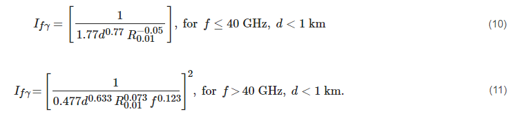
| [42][52] | r=⎧⎩⎨⎪⎪⎪⎪⎪⎪⎪⎪[11.77d0.77R−0.050.01][10.477d0.633R0.0730.01f0.123]2f≤40GHzf>40GHz | It was based on the measured attenuation of smaller than 1 km terrestrial link and frequency 26/38 GHz. | It concluded that the distance factor is inconsistent for a link length smaller than 1 km. |
⧫ m(F,l)=1+Ψ(F)lnl and Ψ(F)=1.4×10⁻⁴F1.76 the value of depends on path length and the considered rain percentage exceedance, ▲ ζ(L)=−100 when L≤7km and ζ(L)=⌈(44.2L)⌉0.78 when L>7km, ♣ ζ0.01=ζ1; R0.01≥110mm/h, otherwise ζ0.01=S2 or ζ2S3
Table 4.
| Ref. | Technique or Resolution | Remarks |
|---|
| [43][53] | E=1nCountry∑i=1415Wi∣∣∣log(RiDBSG3RiS−B)∣∣∣ | This test was used to re-analysis based rain rate and the rain rate provided by the ITU-R DBSG3 database. |
| [44][54] | ER0.01=E2ψ+E2ϕ+ΔR0.012−−−−−−−−−−−−−−−√ where E2ψ=(∂R0.01∂ψ)2σ2ψ and E2ϕ=(∂R0.01∂ϕ)2σ2ϕ. |
The model was developed and verified using DBGS3 along with CHIRPS rainfall (ψ), and TPW (ϕ) in the ERA-Interim Reanalysis database. Authors have not compared with measured data and the precise calculation of rain rate R0.01 showed lower accuracy (uncertainty is about 14%). |
A rain-rate-retrieval algorithm was designed using radar reflectivity derived from the rain rate in [45]. Based on the Doppler velocity, the derived radar reflectivity was classified as low-and high-rain cases. This model paved the way for blending reflectivity and attenuation to predict the rain rate. However, beyond reflectivity and attenuation, other factors, such as seasonal variation and rain type, were not considered.
commercial microwave link (CML) within a fixed interval [46]. Using these minima and maxima, the observed attenuation value averaged rain intensity can be calculated as
 R¯¯¯i=(max(Ar_maxi−B,0)α˜L)−−−−−−−−−−−−−−−−−−−−⎷b,
Since 2000, numerical weather prediction (NWP) has become popular in predicting rainfall and has drawn interest from the meteorological forecasting industries, researchers, and other stakeholders. However, owing to decreased portability and implementation coverage in remote locations, NWP-based techniques are not a potential technique for remote area application. Therefore, the prediction of learning supported rain diminution is standard because the problem of the NWP technique can be solved. In [47][48][49][50][51][52][53] ML-based rainfall prediction techniques were presented.
1.3. Distance Correction
A
 A=γLe.
Assuming the effective path length
Le
 Le=Aγ.
Owing to the non-uniform distribution of rain, the values of the specific and link attenuation (for 1 km length) are different, which defines a term called the effective path length. This implies that the effectual and actual distance varies for non-uniform rain distributions and links. The effectual distance is usually calculated based on the rainfall distribution [2]. Many models calculate the effective path length using a correction factor, referred to as the path adjustment factor. In terrestrial links, all the link lengths remain within a single rain cell for a short link or many cells for a long link. A brief discussion on the parameters that affect either the effective path length or path length adjustment factor is presented in the next section. In most cases, the accuracy of the model discussed above was calculated using the measured rain attenuation data, which was then compared to the attenuation derived through the attenuation formula. In some cases, the root means square (RMS) and standard deviation (STD) values were calculated to validate the model.
1.4. Frequency and Polarization
The specific attenuation can be determined from the rainfall rate, frequency and polarization using the following power-law relation[19][54][55] .
1.4. Frequency and Polarization
 Asp(dB/km)=xRy0.01,
where
R0.01 is the rain rate, and x and y are regression coefficients that depend on several factors such as: polarization, carrier frequency, temperature, and rain drop size distribution[54] . The values of x and y can be determined experimentally as empirical values. ITU-R P. 838-3[19], provides the prediction values for x and y for 1–100 GHz frequency bands at horizontal and vertical polarizations.In this section, various parameters of rain attenuation, rain rate data collection procedure, available public domain databases, time-series generation techniques, percentage of time exceedance of rain (Equation (
7)), specific attenuation coefficient determination procedure, and the procedure of distance correction factor have been discussed. All the data collected or modified through these techniques can be used by the rain attenuation models, which will be discussed in the next section.
2. Rain Attenuation Models: Terrestrial Links
- Optimization-based model:
- In this type of model, the input parameters of some of the other factors that affect the rain attenuation are developed through optimization (e.g., minimum error value) process.
-
Empiricalmodel: The model is based on experimental data observations rather than input-output relationships that can be mathematically described. The model is then classified as an empirical category.
-
Physical model: The physical model is based on some of the similarities between the rain attenuation model’s formulation and the physical structure of rain events.
-
Statistical model: This approach is based on statistical weather and infrastructural data analysis, and the final model is built as a result of regression analysis in most cases.
-
Fade slope model: In the fade slope model, the slope of attenuation from the rain attenuation versus time data was developed with a particular experimental setup. Later, these data were used to predict rain attenuation.
-
Optimization-based model: In this type of model, the input parameters of some of the other factors that affect the rain attenuation are developed through optimization (e.g., minimum error value) process.
-
Empiricalmodel: The model is based on experimental data observations rather than input-output relationships that can be mathematically described. The model is then classified as an empirical category.
-
Physical model: The physical model is based on some of the similarities between the rain attenuation model’s formulation and the physical structure of rain events.
-
Statistical model: This approach is based on statistical weather and infrastructural data analysis, and the final model is built as a result of regression analysis in most cases.
-
Fade slope model: In the fade slope model, the slope of attenuation from the rain attenuation versus time data was developed with a particular experimental setup. Later, these data were used to predict rain attenuation.
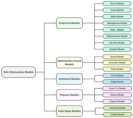
Figure 1.
2.1. Empirical Models
2.1.1. Moupfouma Model
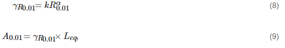
This model [35] uses the rain rate exceeded by 0.01 percent of the time and the calculation of the proportion of time-correlated with the excess of any given interest attenuation.
where
Leq is the equivalent path length for which the rain propagation is assumed to be uniform.
2.1.2. Budalal Model
In this model [42] according to the 300 m link’s attenuation analysis with frequencies of 26 and 38 GHz, the authors found attenuation inconsistency provided by the latest ITU-R model. They then investigate the specific attenuation (
γth) as per ITU-R P.838-3 [19] and found an inconsistency between the effective specific attenuation (
γeff
2.1.3. Perić Model
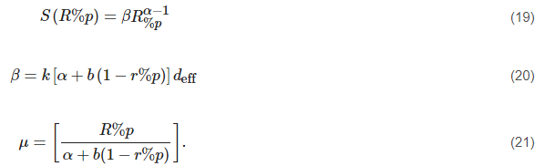
This model is also referred to as a dynamic model [56]. It depends on the cumulative distribution function of the rain intensity of the area of interest, the number of rain events in which the rain intensity threshold is exceeded, the rain advection vector intensity, and the rain advection vector azimuth. The model considers the spatial distribution within a 10 km radius around an antenna and is suitable for small geographical areas, up to 10 km × 10 km. Furthermore, it has not been tested in a real-world network environment.
2.1.4. Garcia Model
It is one of the modified version [57] of Lin model [32], assuming that the
path length reduction coefficient

2.1.5. Da Silva/Unified Model
This model [58] uses the full rainfall rate distribution with multiple nonlinear regressions from the rain attenuation database. It is primarily developed for terrestrial links and can be later extended to slant links. For a terrestrial link,

where
ReffT
d0
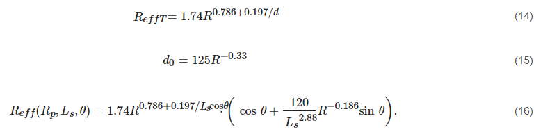
Ls=d
θ=0∘
2.1.6. Mello Model
According to this model[59] the cumulative probability distribution of rain attenuation for terrestrial link can be determined by the Equation (
According to this model [69] the cumulative probability distribution of rain attenuation for terrestrial link can be determined by the Equation ():
2.1.7. Abdulrahman Model

2.1.8. Crane Model
This model [61] establishes rain distribution from a global perspective and the USA’s precise rain distribution maps. From these maps, the rain rate distribution can be calculated.
If the path length
If the path lengthD>22.5km
, then the rain rate should be modified: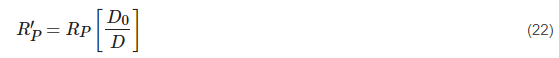
where
whereD0=22.5km
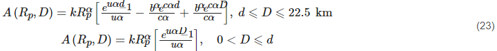
where the constants are given by Equation (
where the constants are given by Equation ()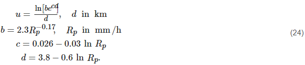
2.2. Physical Models
2.2.1. Crane Two-Component (T-C) Model
This model [62] is based on different integration techniques for heavy and light rainfall regions. The author proposed two versions of the T-C models: the first is a simple T-C model and was published in 1982. The model consisted of several steps. (1) Determining the propagation path for the global climate. (2) Finding a mathematical relation between the projected path length in the rain cell and debris region. (3) Fixing the expected amount of attenuation. (4) Deriving the required rain rate to produce rain attenuation and calculating the probability that the specified attenuation is fixed in step (3).

debris
cell
2.2.2. Ghiani Model
This model [63] is based on a PCF-correction-based model for terrestrial links. It can be modeled by simulation with Equation (
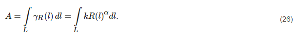 A=∫LγR(l)dl=∫LkR(l)αdl.
 A=kRTXαLPF.
PCF=A/kRTXαL

a
b
c
 A(P,L)=kR(P)αL[a(L)e−b(L)R+c(L)],
where the constants are given by the set of equations in (
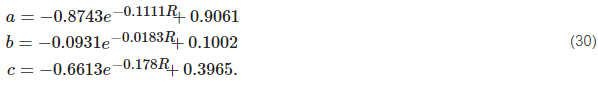 a=−0.8743e−0.1111R+0.9061b=−0.0931e−0.0183R+0.1002c=−0.6613e−0.178R+0.3965.
2.2.3. Excell/Capsoni Model
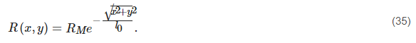
The parameters of this statistical model [64] of the horizontal rain structure can be determined based on the local statistical distribution of the point rainfall intensity. The model was validated using the COST 205, 1985 database. This model consists of several rain cell structures, collectively refereed to as kernels. In such a rain cell, the rainfall rate at a distance
l
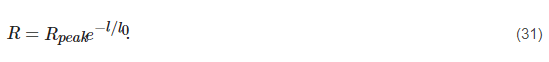 R=Rpeake−l/l0.
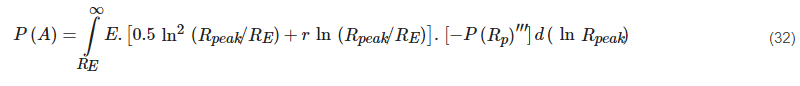
where
r=1/4πl¯0
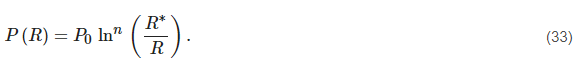
P(R)=0

along a cell radius:
In the sense of the rain attenuation model, this model does not provide attenuation. However, it facilitates the generation of a synthetic rain rate from which attenuation can be predicted using a suitable prediction model. There are critics that the exponential rain peak is not present [65] in nature, and the model does not differentiate between stratiform and convective rain.
2.3. Statistical Models
2.3.1. ITU-R Model
This model [40] is primarily based on a distance factor that relies on the rain rate
R0.01
α
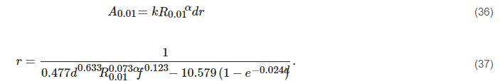
Ap
p
A0.01. This model, validated in Malaysia, showed good agreement with the measured attenuation [66].
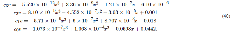
2.3.2. Singh Model
This model [67] provides an easy calculation mechanism compared to the ITU-R model. The specific attenuation follows the ITU-R model for the frequency band of 1–100 GHz. After calculating the specific attenuation, the curve fitting technique using the MATLAB software cubic polynomial Equation (

where the coefficients
c3
c2
c1
c0
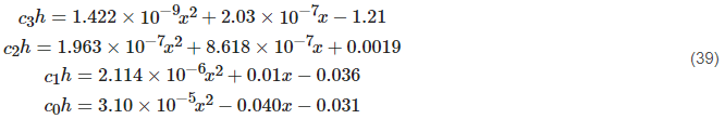
and for the vertical polarization:
A similar approach-based technique was proposed in[68] . However, it was considered the original power-law relationship rather than the simplified polynomial form in that proposal. The second difference is that the constants
A similar approach-based technique was proposed in [78]. However, it was considered the original power-law relationship rather than the simplified polynomial form in that proposal. The second difference is that the constantsk
,α
referring to the Equation () depends only on frequency and either vertical or horizontal polarization.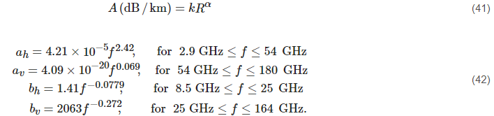
2.4. Fade Slope Models
2.4.1. Andrade Model
In the Andrade model [69] the variance of the fade slope is proportional to the attenuation as per Equation (
A(ti+tp)
A(ti)

where
tp
tp=10
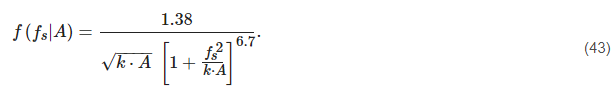
2.4.2. Chebil Model
In the Chebil model[5] the variance of the fade slope is proportional to the attenuation as per Equation (
In the Chebil model [16] the variance of the fade slope is proportional to the attenuation as per Equation (): p(ξ∣A)=1σξ2π−−√exp(0.5(ξσξ)2),
where the
where theσξ
is given by Equation ()
2.5. Optimization-Based Models
2.5.1. Develi Model
This model [70] is based on the Differential evolution approach (DEA) optimization technique and experimentally tested at 97 GHz on terrestrial link in the United Kingdom (UK). The steps of the DEA attenuation model are as follows:
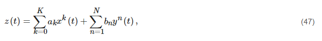
where
ak,bn
k=0,1,…,K
n=1,2,…,N
K+N
which can be alternatively represented as:


where
n
Pmut
p1,p2
i
M
opt
gene pool
optimal entity
2.5.2. Livieratos Model
This model [71] was developed using a DBSG3 database-based on a supervised machine-learning (SML) technique. In this rain attenuation model, the SML technique was blended with a Gaussian process (GP). A rain attenuation algorithm must be trained in a particular area of interest to measure the different interdependencies of the parameters for detecting rain attenuation in a specific region, weather, or carrier frequency.
2.5.3. Pinto Model
This model [72] is based on the actual distance correction mechanism through the distance correction factor (
r
Reff

ai(i=1,2,…,9) coefficients can be calculated using quasi-Newton multiple nonlinear regression (QNMRN) and the Gaussian RMSE (GRMSE) algorithm. These coefficients were further fine-tuned using the PSO technique. The model performance has not been compared with the recently developed model, except for ITU-R P.530-17 [40]. Thus, there is a need for further verification before application, except for the temperate climate and Malaysia rainfall database areas.