A watershed is defined by natural topographic boundaries as an ecosystem of integrated terrestrial and aquatic systems, rather than the political boundaries, in which all of the incoming precipitation and snowmelt are collected into the stream reaches while a river basin is an area of land drained by a river, its tributaries and watersheds.
- watershed modeling
- cold climate
- climate change
- modeling of river basins
1. Introduction
A watershed is defined by natural topographic boundaries as an ecosystem of integrated terrestrial and aquatic systems, rather than the political boundaries, in which all of the incoming precipitation and snowmelt are collected into the stream reaches while a river basin is an area of land drained by a river, its tributaries and watersheds. The watershed function is generally defined as its response to the water entering its control volume [10,22][1][2]. The river shape, land topology, wetlands and riparian zones regulate the overland and subsurface flows as well as groundwater. Water budget in a watershed is balanced by precipitation, evapotranspiration, infiltration, and runoff. For a cold region, glacier, snowpack, permafrost, etc. (frozen water components) are also important parts of water budget. Some of the models discussed in this paper may not have a good process to capture those budgets. Watershed ecosystems are controlled by a suite of hierarchically nested physical, chemical, and biological processes operating over space and time.
A watershed consists of terrestrial or aquatic sub-ecosystems, including forest, grasslands, arable, urban, and wetlands. Water, energy, air, vegetation and land interact within the watershed. Some main watershed processes can be broken down into specific functions and characteristics, including hydrological processes (i.e., overland flow, evaporation, infiltration, groundwater recharge, and erosion), biogeochemical processes (i.e., nutrient cycling, pollution transport and fate, mineralization and organic matter decomposition), and land-surface interaction (i.e., plant growth, photosynthesis, and evapotranspiration). In cold regions, there are four special elements, including snow, permafrost, freeze-thaw cycle and glaciers as well as lake and river ices (Figure 1) [12][3]. The biogeochemical processes, such as nitrification, denitrification and decomposition, can be affected by soil water, temperature and pH, depending on various hydrological processes. Human activities, such as land use changes, mining and water policy can also affect water balance and biogeochemical processes. Intensive agricultural practices, such as grazing, irrigation and fertilization, can affect hydrological and biogeochemical processes, and cause land degradation, such as salinization and desertification [21][4].
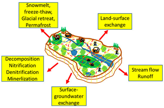
Figure 1. Watershed ecosystem processes at larger spatial scales (heavy arrows).
2. Principles of Watershed Modelling
Watershed modeling is to quantify hydrology and biogeochemistry with associated ecosystem functions, such as plant dynamics, in the watershed. An ideal basin-oriented strategy is to simulate the integration of watershed hydrology, nutrient, and sediment reactive transport below and above ground [23][5]. However, in reality, we cannot include all detailed watershed processes. Hence, abstraction through parameterization and simplification is necessary in representing complexity level of watershed system and processes. The parameterization and simplification are a compromise between reality, feasibility, and simplicity in a watershed model and are to use some replacement of watershed processes using a model of similar but simpler, more empirical conceptual structure. The point is not a perfect solution but a replacement to reflect the physical reality as good as possible. Thus, a watershed model is an approximation of its reality to describe the watershed processes and system which can retain most of its important characteristics [13,24][6][7].
Conceptually, it is quite natural to use a symbolic watershed model to represent some of the natural hydrological and biogeochemical processes of the real system according to the first principle. A set of equations of mass, momentum, and energy conservation along with initial and boundary conditions can be established to describe the streamflow, infiltration, subsurface flow, and baseflow in a watershed system driven by the weather conditions, such as precipitation and solar radiation, soil and plants. Unfortunately, these equations cannot be solved analytically and can be solved only for very simple geometries or boundary conditions. Therefore, a watershed domain is usually distributed on discrete grids and the partial differential equations are replaced by their discrete equations. For example, the Richards equation of water transport in soil are solved by using finite difference method [25,26,27,28,29][8][9][10][11][12]. However, such models require extensive data and physical parameter, which may not be efficient to set up the model. Furthermore, a watershed model needs to consider readily available data with sufficient efficiency of computer power and memory while simulating large river basins. This will allow realistic simulation of some medium complexity, which generally includes relatively detailed data inputs such as topography, land use, soil, weather, and water quality. Thus, many distributed models delineate a watershed into a multi-level hierarchically distributed drainage system using reasonable spatial discrete elements, such as sub-basins and hydrological response units (HRUs) in SWAT [30][13], CRHM [19][14] and HSPF [31][15], and a grid of large (>>1 km), flat, uniform cells in the VIC (Table 1). These watershed models not only represent the fundamental water and sediment transport processes, but also combine the empirical and statistical equations such as nitrification, denitrification and decomposition. The use of the lumped parameters and HRUs or similar units are to reduce the grid number because the computational cost depends on the numbers of grid cells and parameters [32][16].
Characteristics of watershed models in cold regions.
| Model Name | Spatial Resolution | Time Step | Snowpack Model | Snowpack Layer | Water Quality | GHGs | References |
|---|---|---|---|---|---|---|---|
| HSPF | HRUs | Sub-daily | Snowmelt/sublimation/ compaction/albedo/blowing/radiation/interception | Two layers | Yes | [18,33,34] | |
| CRHM | HRUs | Daily | Snowmelt/sublimation/ compaction/albedo/blowing/radiation/interception | Two layers | [19,35][14] | ||
| CRHM+ WINTRA | HRUs | Daily | Snowmelt/sublimation/ compaction/albedo/blowing/radiation/interception | Two layers | Yes | [36,37] | |
| SWAT | HRUs | Daily | Snowmelt/sublimation | One layer | Yes | [15,38,39,40,41] | |
| VIC | Grid cell (>>1 km2) |
Daily | Snowmelt/sublimation/ compaction/albedo/blowing/radiation/interception | Two layers | Yes | [42,43] | |
| SWAT-DayCent | HRUs | Daily | Snowmelt/sublimation | One layer | Yes | N2O/CO2 | [44,45,46,47,48] |
| SWAT-MKT | HRUs | Daily | Snowmelt/sublimation | One layer | Yes | N2O/CO2/NEE | [49,50,51] |
| VIC-CropSyst | Grid cell (>>1 km2) |
Daily | Snowmelt/sublimation/ compaction/albedo/blowing/radiation/interception | Two layers | Yes | [52,53,54] |
In every HRU unit, the parameters of a watershed model represent a volume-average of their variability over the unit that consists of homogeneous land use, management and soil properties, slopes and weather conditions. In the HRUs, only percentages of the land uses are represented, and parameters, such as soil properties and land uses are not identified spatially in these models [30]. For example, in the VIC model, the sub-grid variability is handled in terms of statistical properties [30,42,55]. Therefore, land-atmosphere fluxes, and the water and energy balances are calculated at a daily or sub-daily time step but horizontal flow between HRUs is not considered [30,42]. The water balance is calculated among rainfall, runoff, infiltration, evapotranspiration, storage, snowmelt water, lateral subsurface flow from the soil layers and baseflow at each HRU. Flows are aggregated from all HRUs to the sub-basin level, and then directed to stream reaches along the directions of element slopes using either the variable-rate storage method or the Muskingum method [19,56]. Sediment, nutrient, pollutants, and bacteria loading from each HRU are also collected at the subbasin outlets, and are directed to channels, ponds, wetlands, and lakes. Contributions from point sources and urban areas can be inputted from HRUs and be exported from each sub-basin.
Reference (Editors will rearrange the references after the entry is submitted)
- Shrestha, N.K.; Du, X.; Wang, J. Assessing climate change impacts on fresh water resources of the Athabasca River Basin, Canada. Sci. Total. Environ. 2017, 601–602, 425–440.
- Shrestha, N.K.; Wang, J. Predicting sediment yield and transport dynamics of a cold climate region watershed in changing climate. Sci. Total. Environ. 2018, 625, 1030–1045.
- Du, X.; Goss, G.; Faramarzi, M. Impacts of hydrological processes on stream temperature in a cold region watershed based on the SWAT Equilibrium Temperature model. Water 2020, 12, 1112.
- Barnett, T.P.; Adam, J.C.; Lettenmaier, D.P. Potential impacts of a warming climate on water availability in snow-dominated regions. Nature 2005, 438, 303–309.
- Bennett, K.E.; Werner, A.T.; Schnorbus, M. Uncertainties in hydrologic and climate change impact analyses in headwater basins of British Columbia. J. Clim. 2012, 25, 5711–5730.
- IPCC. Climate Change 2007: Impacts, Adaptation and Vulnerability. Contribution of Working Group II to the Fourth Assessment Report of the Intergovernmental Panel on Climate Change; Cambridge University Press: Cambridge, UK, 2007.
- Darghouth, S.; Ward, C.; Gambarelli, G.; Styger, E.; Roux, J. Watershed Management Approaches, Policies, and Operations: Lessons for Scaling Up; The World Bank: Washington, DC, USA, 2008.
- IPCC. Climate Change 2014: Synthesis Report. Contribution of Working Groups I, II, and III to the Fifth Assessment Report of the In-tergovernmental Panel on Climate Change; IPCC: Geneva, Switzerland, 2014.
- Loiselle, D.; Du, X.; Alessi, D.S.; Bladon, K.D.; Faramarzi, M. Projecting impacts of wildfire and climate change on streamflow, sediment, and organic carbon yields in a forested watershed. J. Hydrol. 2020, 590, 125403.
- Chen, X.; Lee, R.M.; Dwivedi, D.; Son, K.; Fang, Y.; Zhang, X.; Graham, E.; Stegen, J.; Fisher, J.B.; Moulton, D.; et al. Integrating field observations and process-based modeling to predict watershed water quality under environmental perturbations. J. Hydrol. 2020, 125762, 125762.
- Vuille, M.; Carey, M.; Huggel, C.; Buytaert, W.; Rabatel, A.; Jacobsen, D.; Soruco, A.; Villacis, M.; Yarleque, C.; Timm, O.E.; et al. Rapid decline of snow and ice in the tropical Andes—Impacts, uncertainties and challenges ahead. Earth Sci. Rev. 2018, 176, 195–213.
- Hock, R.; Rasul, G.; Adler, C.; Cáceres, B.; Gruber, S.; Hirabayashi, Y.; Jackson, M.; Kääb, A.; Kang, S.; Kutuzov, S.; et al. High mountain areas. In IPCC Special Report on the Ocean and Cryosphere in a Changing Climate. Pörtner, H.-O., Roberts, D.C., Masson-Delmotte, V., Zhai, P., Tignor, M., Poloczanska, E., Mintenbeck, K., Alegría, A., Nicolai, M., Okem, A., et al., Eds.; IPCC: Geneva, Switzerland, 2019; in press.
- Singh, V.P.; Woolhiser, D.A. Mathematical modeling of watershed hydrology. J. Hydrol. Eng. 2002, 7, 270–292.
- Joshi, R.; Kumar, K.; Adhikari, V.P.S. Modelling suspended sediment concentration using artificial neural networks for Gangotri glacier. Hydrol. Process. 2016, 30, 1354–1366.
- Arnold, J.G.; Srinivasan, R.; Muttiah, R.S.; Williams, J.R. Large area hydrologic modeling and assessment part i: Model development. J. Am. Water Resour. Assoc. 1998, 34, 73–89.
- Arnold, J.G.; Moriasi, D.N.; Gassman, P.W.; Abbaspour, K.C.; White, M.J.; Srinivasan, R.; Santhi, C.; Harmel, R.D.; Van Griensven, A.; Van Liew, M.W.; et al. SWAT: Model use, calibration, and validation. Am. Soc. Agric. Biol. Eng. 2012, 55, 1491–1508.
- Eum, H.-I.; Dibike, Y.; Prowse, T. Comparative evaluation of the effects of climate and land-cover changes on hydrologic responses of the Muskeg River, Alberta, Canada. J. Hydrol. Reg. Stud. 2016, 8, 198–221.
- Bicknell, B.R.; Imhoff, J.C.; Kittle, J.L.J.; Donigian, A.S.J.; Johanson, R.C. Hydrological Simulation Program—Fortran, User’s manual for version 11; U.S. Environmental Protection Agency, National Exposure Research Laboratory: Athens, GA, USA, 1997.
- Pomeroy, J.W.; Gray, D.M.; Brown, T.; Hedstrom, N.R.; Quinton, W.L.; Granger, R.J.; Carey, S.K. The cold regions hydrological model: A platform for basing process representation and model structure on physical evidence. Hydrol. Process. 2007, 21, 2650–2667.
- Zhou, G.; Wei, X.; Wu, Y.; Liu, S.; Huang, Y.; Yan, J.; Zhang, D.; Zhang, Q.; Liu, J.; Meng, Z.; et al. Quantifying the hydrological responses to climate change in an intact forested small watershed in Southern China. Glob. Chang. Biol. 2011, 17, 3736–3746.
- Wang, J.; Li, Y.; Bork, E.W.; Richter, G.M.; Eum, H.-I.; Chen, C.; Shah, S.H.H.; Mezbahuddin, S. Modelling spatio-temporal patterns of soil carbon and greenhouse gas emissions in grazing lands: Current status and prospects. Sci. Total. Environ. 2020, 739, 139092.
- Wagener, T.; Sivapalan, M.; Troch, P.; Woods, R. Catchment classification and hydrologic similarity. Geogr. Compass 2007, 1, 901–931.
- Nash, J.E.; Sutcliffe, J.V. River flow forecasting through conceptual models part I—A discussion of principles. J. Hydrol. 1970, 10, 282–290.
- Woolhiser, D.A. Hydrologic and Watershed Modeling-State of the Art. Trans. ASAE 1973, 16, 553–559.
- Yeh, G.-T.; Shih, D.-S.; Cheng, J.-R.C. An integrated media, integrated processes watershed model. Comput. Fluids 2011, 45, 2–13.
- Ma, L.; He, C.; Bian, H.; Sheng, L. MIKE SHE modeling of ecohydrological processes: Merits, applications, and challenges. Ecol. Eng. 2016, 96, 137–149.
- Deng, B.; Wang, J. Saturated-unsaturated groundwater modeling using 3D Richards equation with a coordinate transform of nonorthogonal grids. Appl. Math. Model. 2017, 50, 39–52.
- Langevin, C.D.; Hughes, J.D.; Banta, E.R.; Niswonger, R.G.; Sorab, P.; Provost, A.M. Documentation for the MODFLOW 6 Groundwater Flow Model. In U.S. Geological Survey Techniques and Methods; Book 6; U.S. Geological Survey: Reston, VA, USA, 2017.
- Orgogozo, L.; Renon, N.; Soulaine, C.; Hénon, F.; Tomer, S.; Labat, D.; Pokrovsky, O.; Sekhar, M.; Ababou, R.; Quintard, M. An open source massively parallel solver for Richards equation: Mechanistic modelling of water fluxes at the watershed scale. Comput. Phys. Commun. 2014, 185, 3358–3371.
- Gassman, P.W.; Reyes, M.R.; Green, C.H.; Arnold, J.G. The soil and water assessment tool: Historical development, applications, and future research directions. Trans. ASABE 2007, 50, 1211–1250.
- Skahill, B.E. Use of the Hydrological Simulation Program—FORTRAN (HSPF) Model for Watershed Studies; ERDC/TN SMART-04-1; Army Engineer Research and Development Center: Vicksburg, MS, USA, 2004.
- Wang, J.; Zhang, X.; Bengough, A.G.; Crawford, J.W. Domain-decomposition method for parallel lattice Boltzmann simulation of incompressible flow in porous media. Phys. Rev. E 2005, 72, 016706.
- Crossette, E.; Panunto, M.; Kuan, C.; Mohamoud, Y.M. Application of the BASINS/HSPF to Data Scare Watersheds; U.S. Environmental Protection Agency: Washington, DC, USA, 2015.
- Seong, C.; Her, Y.; Benham, B.L. Automatic calibration tool for hydrologic simulation program-FORTRAN using a shuffled complex evolution algorithm. Water 2015, 7, 503–527.
- Ellis, C.R.; Pomeroy, J.W.; Brown, T.; Macdonald, J. Simulation of snow accumulation and melt in needleleaf forest environments. Hydrol. Earth Syst. Sci. 2010, 14, 925–940.
- Costa, D.; Roste, J.; Pomeroy, J.; Baulch, H.; Elliott, J.; Wheater, H.; Westbrook, C. A modelling framework to simulate field-scale nitrate response and transport during snowmelt: The WINTRA model. Hydrol. Process. 2017, 31, 4250–4268.
- Costa, D.; Pomeroy, J.; Baulch, H.; Elliott, J.; Wheater, H. Using an inverse modelling approach with equifinality control to investigate the dominant controls on snowmelt nutrient export. Hydrol. Process. 2019, 33, 2958–2977.
- Shrestha, N.K.; Wang, J. Water Quality management of a cold climate region watershed in changing climate. J. Environ. Informatics 2020, 35, 56–80.
- Du, X.; Shrestha, N.K.; Wang, J. Incorporating a non-reactive heavy metal simulation module into SWAT model and its application in the Athabasca oil sands region. Environ. Sci. Pollut. Res. 2019, 26, 20879–20892.
- Du, X.; Shrestha, N.K.; Wang, J. Integrating organic chemical simulation module into SWAT model with application for PAHs simulation in Athabasca oil sands region, Western Canada. Environ. Model. Softw. 2019, 111, 432–443.
- Meshesha, T.W.; Wang, J.; Melaku, N.D. A modified hydrological model for assessing effect of pH on fate and transport of Escherichia coli in the Athabasca River basin. J. Hydrol. 2020, 582, 124513.
- Liang, X.; Lettenmaier, D.P.; Wood, E.F.; Burges, S.J. A simple hydrologically based model of land surface water and energy fluxes for general circulation models. J. Geophys. Res. Atmos. 1994, 99, 14415–14428.
- Eum, H.-I.; Dibike, Y.; Prowse, T. Climate-induced alteration of hydrologic indicators in the Athabasca River Basin, Alberta, Canada. J. Hydrol. 2017, 544, 327–342.
- Wagena, M.B.; Bock, E.M.; Sommerlot, A.R.; Fuka, D.R.; Easton, Z.M. Development of a nitrous oxide routine for the SWAT model to assess greenhouse gas emissions from agroecosystems. Environ. Model. Softw. 2017, 89, 131–143.
- Shrestha, N.K.; Wang, J. Modelling nitrous oxide (N2O) emission from soils using the Soil and Water Assessment Tool (SWAT). In Proceedings of the 2018 SWAT Conference, Chennai, India, 10–12 January 2018.
- Shrestha, N.K.; Wang, J. Current and future hot-spots and hot-moments of nitrous oxide emission in a cold climate river basin. Environ. Pollut. 2018, 239, 648–660.
- Melaku, N.D.; Shrestha, N.K.; Wang, J.; Thorman, R.E. Predicting nitrous oxide emissions after the application of solid manure to grassland in the United Kingdom. J. Environ. Qual. 2020, 49, 1–13.
- Melaku, N.D.; Wang, J.; Meshesha, T.W. Improving hydrologic model to predict the effect of snowpack and soil temperature on carbon dioxide emission in the cold region peatlands. J. Hydrol. 2020, 587, 124939.
- Bhanja, S.N.; Wang, J. Estimating influences of environmental drivers on soil heterotrophic respiration in the Athabasca River Basin, Canada. Environ. Pollut. 2020, 257, 113630.
- Bhanja, S.N.; Wang, J.; Shrestha, N.K.; Zhang, X. Modelling microbial kinetics and thermodynamic processes for quantifying soil CO2 emission. Atmospheric Environ. 2019, 209, 125–135.
- Bhanja, S.N.; Wang, J.; Shrestha, N.K.; Zhang, X. Microbial kinetics and thermodynamic (MKT) processes for soil organic matter decomposition and dynamic oxidation-reduction potential: Model descriptions and applications to soil N2O emissions. Environ. Pollut. 2019, 247, 812–823.
- Stöckle, C.O.; Donatelli, M.; Nelson, R. CropSyst, a cropping systems simulation model. Eur. J. Agron. 2003, 18, 289–307.
- Stöckle, C.O.; Kemanian, A.R.; Nelson, R.L.; Adam, J.C.; Sommer, R.; Carlson, B. CropSyst model evolution: From field to regional to global scales and from research to decision support systems. Environ. Model. Softw. 2014, 62, 361–369.
- Adam, J.C.; Stephens, J.C.; Chung, S.H.; Brady, M.P.; Evans, R.D.; Kruger, C.E.; Lamb, B.K.; Liu, M.; Stöckle, C.O.; Vaughan, J.K.; et al. BioEarth: Envisioning and developing a new regional earth system model to inform natural and agricultural resource management. Clim. Chang. 2015, 129, 555–571.
- Krysanova, V.; Arnold, J.G. Advances in ecohydrological modelling with SWAT—a review. Hydrol. Sci. J. 2008, 53, 939–947.
- Neitsch, S.L.; Arnold, J.G.; Kiniry, J.R.; Williams, J.R. Soil & Water Assessment Tool Theoretical Documentation; Version 2009; Grassland, Soil and Water Research Laboratory-Agricultural Research Service, Blackland Research Center-Texas AgriLife Research: Temple, TX, USA, 2011.
References
- Chen, X.; Lee, R.M.; Dwivedi, D.; Son, K.; Fang, Y.; Zhang, X.; Graham, E.; Stegen, J.; Fisher, J.B.; Moulton, D.; et al. Integrating field observations and process-based modeling to predict watershed water quality under environmental perturbations. J. Hydrol. 2020, 125762, 125762.
- Wagener, T.; Sivapalan, M.; Troch, P.; Woods, R. Catchment classification and hydrologic similarity. Geogr. Compass 2007, 1, 901–931.
- Hock, R.; Rasul, G.; Adler, C.; Cáceres, B.; Gruber, S.; Hirabayashi, Y.; Jackson, M.; Kääb, A.; Kang, S.; Kutuzov, S.; et al. High mountain areas. In IPCC Special Report on the Ocean and Cryosphere in a Changing Climate. Pörtner, H.-O., Roberts, D.C., Masson-Delmotte, V., Zhai, P., Tignor, M., Poloczanska, E., Mintenbeck, K., Alegría, A., Nicolai, M., Okem, A., et al., Eds.; IPCC: Geneva, Switzerland, 2019; in press.
- Wang, J.; Li, Y.; Bork, E.W.; Richter, G.M.; Eum, H.-I.; Chen, C.; Shah, S.H.H.; Mezbahuddin, S. Modelling spatio-temporal patterns of soil carbon and greenhouse gas emissions in grazing lands: Current status and prospects. Sci. Total. Environ. 2020, 739, 139092.
- Nash, J.E.; Sutcliffe, J.V. River flow forecasting through conceptual models part I—A discussion of principles. J. Hydrol. 1970, 10, 282–290.
- Singh, V.P.; Woolhiser, D.A. Mathematical modeling of watershed hydrology. J. Hydrol. Eng. 2002, 7, 270–292.
- Woolhiser, D.A. Hydrologic and Watershed Modeling-State of the Art. Trans. ASAE 1973, 16, 553–559.
- Yeh, G.-T.; Shih, D.-S.; Cheng, J.-R.C. An integrated media, integrated processes watershed model. Comput. Fluids 2011, 45, 2–13.
- Ma, L.; He, C.; Bian, H.; Sheng, L. MIKE SHE modeling of ecohydrological processes: Merits, applications, and challenges. Ecol. Eng. 2016, 96, 137–149.
- Deng, B.; Wang, J. Saturated-unsaturated groundwater modeling using 3D Richards equation with a coordinate transform of nonorthogonal grids. Appl. Math. Model. 2017, 50, 39–52.
- Langevin, C.D.; Hughes, J.D.; Banta, E.R.; Niswonger, R.G.; Sorab, P.; Provost, A.M. Documentation for the MODFLOW 6 Groundwater Flow Model. In U.S. Geological Survey Techniques and Methods; Book 6; U.S. Geological Survey: Reston, VA, USA, 2017.
- Orgogozo, L.; Renon, N.; Soulaine, C.; Hénon, F.; Tomer, S.; Labat, D.; Pokrovsky, O.; Sekhar, M.; Ababou, R.; Quintard, M. An open source massively parallel solver for Richards equation: Mechanistic modelling of water fluxes at the watershed scale. Comput. Phys. Commun. 2014, 185, 3358–3371.
- Gassman, P.W.; Reyes, M.R.; Green, C.H.; Arnold, J.G. The soil and water assessment tool: Historical development, applications, and future research directions. Trans. ASABE 2007, 50, 1211–1250.
- Pomeroy, J.W.; Gray, D.M.; Brown, T.; Hedstrom, N.R.; Quinton, W.L.; Granger, R.J.; Carey, S.K. The cold regions hydrological model: A platform for basing process representation and model structure on physical evidence. Hydrol. Process. 2007, 21, 2650–2667.
- Skahill, B.E. Use of the Hydrological Simulation Program—FORTRAN (HSPF) Model for Watershed Studies; ERDC/TN SMART-04-1; Army Engineer Research and Development Center: Vicksburg, MS, USA, 2004.
- Wang, J.; Zhang, X.; Bengough, A.G.; Crawford, J.W. Domain-decomposition method for parallel lattice Boltzmann simulation of incompressible flow in porous media. Phys. Rev. E 2005, 72, 016706.