Recent tests measured an irrotational (curl-free) magnetic vector potential (A) that is contrary to classical electrodynamics (CED). A (irrotational) arises in extended electrodynamics (EED) that is derivable from the Stueckelberg Lagrangian. A (irrotational) implies an irrotational (gradient-driven) electrical current density, J. Consequently, EED is gauge-free and provably unique. EED predicts a scalar field that equals the quantity usually set to zero as the Lorenz gauge, making A and the scalar potential (F) independent and physically-measureable fields. EED predicts a scalar-longitudinal wave (SLW) that has an electric field along the direction of propagation together with the scalar field, carrying both energy and momentum. EED also predicts the scalar wave (SW) that carries energy without momentum.
- scalar-longitudinal wave
- gradient-driven current
- curl-free current
- irrotational current
- gradient-driven current
- curl-free current
- irrotational current
Note: The following contents are extract from your paper. The entry will be online only after author check and submit it.
1. Introduction
Maxwell’s equations are the cornerstone of modern physics, accurately predicting numerous tests and providing the basis for sophisticated 21st century technologies. Classical electrodynamics (CED).is considered to be a firmly established physical theory. Extension of CED to quantum electrodynamics (QED) describes (sub) atomic-scale, matter-light interactions, agreeing with experiments to astounding precision. Thus, mainstream physicists consider CED and QED to be complete and closed with no compelling reason for re-evaluation or alteration. These beliefs arise from the psychological principle of cognitive dissonance that dismisses contrary claims as heretical.
One motivation for this work is that Feynman’s ‘proof’ of Maxell’s equations [1] [1] uses assumptions that make CED inconsistent and incomplete (Section 5). Woodside’s uniqueness proof [2] of extended electrodynamics (EED) makes no such assumptions, yielding Equations (10)–(14). CED lacks the scalar field (C) that leads to new electrodynamic forces and energy terms in Equations (24) and (25), below. Thus, a second motivation for this work is presentation of first-principles theory and recent test results to warrant a thoughtful re-evaluation of CED’s consistency and completeness.
The outline of this paper follows. Section 2 shows that the vector potential (A) is a measureable, physical quantity via theory and compelling experimental evidence. The curl-free (irrotational) vector potential is important in both classical and quantum domains, for example in the Aharonov-Bohm effect and the Maxwell-Lodge effect. We show that A and scalar-potential (F) have the same physical significance as the electric (E) and magnetic (B) fields Section 3 further elucidates A and F, as physically measureable and independent fields for EED theory. Section 4 discusses the EED Lagrangian and scalar field (C). [Note that bold font denotes a 3-dimensional vector (e.g., A, B, E) and italic font denotes scalar quantities (e.g., C)] The centerpiece of this work is Section 5, which presents EED as elucidated by the second author [3]. EED is consistent with preliminary tests [3], showing that an irrotational electrical current drives the scalar longitudinal wave, and includes the missing scalar field for a provably unique EED theory [2]. Section 6 expounds on the SLW’s no-skin-effect constraint, revealing vast applications of EED in new technologies and in natural systems. Section 7 explores the possible future role that EED may play in quantum physics and general relativity. Section 8 presents our conclusions with a discussion of future prospects.
2. Physical Significance of the Magnetic Vector Potential
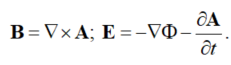
Great controversy surrounds the role of the magnetic vector potential in CED [4][5][6][4-6]. This controversy arises from the fundamental mathematical relationship between the potentials (F and A), and the electric (E) and magnetic (B) fields. B and E can be expressed in terms of F and A, as [7]:
 |
(1) |
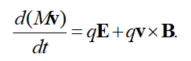
B and E are regarded as physical fields; F and A are viewed as mathematical conveniences for solving Maxwell’s equations. This interpretation arises from the detectability of B and E through the Lorentz-force equation [7] on a point-particle at the position [rq(t)] with a charge (q) and mass (M).:
 |
(2) |
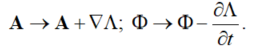
Maxwell’s equations are arbitrary (non-unique) in and under the transformation [8]:
 |
(3) |
The transformation of Equation (3) leaves B and E unchanged in Equation (1), and is termed gauge invariance [8]. Equation (3) allows an À2-infinitude of choices for L. An analyst can choose an appropriate gauge to fix boundary conditions, find the ‘proper’ B and E fields for known charge and current distributions, or solve an inverse problem. This convention is now engrained in CED, but restricts the potentials. For instance, the Lorenz gauge makes the F and A inter-dependent.
The physical significance of the electromagnetic potentials has been debated for decades, as discussed further below. Majumdar and Ray [9][10][9-10] observe that the F- and A-wave equations are non-invertible despite their gauge ambiguity. These wave equations arise from CED via standard Fourier transforms with a unique projection operator that makes a gauge choice superfluous. Nikolova [11] notes that nonzero, radially-propagating (irrotational) potentials occur in antenna theory with zero B- and E-field vectors via expansion of the free-space fields in spherical harmonics. This irrotational “potential wave” is called “longitudinal,” meaning A-polarization in the direction of propagation. The corresponding wave impedance is equal to that of free space. CED predicts that this solution has no radiated power, because the Poynting vector is zero. EED predicts a scalar-longitudinal wave (SLW) with a longitudinal-E field and radiated power (Section 5).
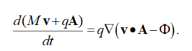
An insightful, under-appreciated dissertation by A. Konopinski [12] elucidates A and its corresponding physical significance in a form that is quite close to that of Faraday [13][14][15][16][17][13-17]. Namely, the vector potential is a “store” of electrodynamic-field momentum available for exchange with the kinetic momentum of charged particles in a conductor [12]. Konopinski shows that operational definitions of F and A arise from Equation (2), in terms of the potentials in Equation (1):
 |
(4) |
This form expresses energy and momentum exchanges without explicit forces. Equation (4) equates the change in “conjugate momentum” (p = Mv + qA) to the negative gradient of “interaction energy,” q(F − v∙A). Konopinski used a novel gedanken-experiment to show that A can be measured everywhere in space. Namely, a charged, macroscopic bead slides freely on a circular, non-conductive fiber that is concentric with the cross-section of a magnetic solenoid. A has only an azimuthal component parallel to the current flow, resulting in ▽F = ▽●A = 0. So, the right-hand side (RHS) of Equation (3) is zero, making the conjugate momentum (p) a conserved quantity. A is obtained by monitoring the associated change in the bead’s kinetic momentum (M v) as the solenoid’s current changes. Then, qA is the conjugate momentum [12] in an external field, just as qF is electrodynamic-field energy per unit charge. These joint properties of the imposed fields arise from their interference and determine the processes, by which fields and charges become observable. Force and power per unit charge are then expressed in terms of the transfer rates.
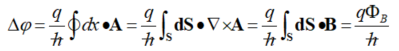
In addition, much experimental evidence validates the irrotational (curl-free) magnetic vector potential in quantum-, meso-, and macro-scale spatial domains, spanning the full electrodynamic frequency spectrum. For example, the Aharonov-Bohm effect (ABE) [18][19][18-19] involves quantum physics of an electrically charged particle (q = charge) via coupling of the scalar (F) and vector (A) potentials with the complex phase of the particle’s wave function. For a particle travelling along a path (P) in a region with zero magnetic field (B) and A≠0, the magnetic phase shift is φ = (q/ħ)ʃP dx●A. Here, ħ is Planck’s constant divided by 2π; ʃP dx is the path integral along the particle’s trajectory. Particles with the same starting and ending points acquire a phase difference (Δφ) by travelling along two distinct paths around a multiply connected domain:
 |
(5) |
The second form is the full path around the multiply connected domain. Use of Stoke’s theorem yields the third form. Substitution of B = ▽ × A gives the fourth form with FB as the enclosed magnetic flux in the fifth form. The wave nature of quantum particles allows the same particle to traverse different paths. Then, the phase difference is observable by placing a magnetic solenoid between the slits of a double-slit experiment. Tests by Tonomura et al. [20] and Osakabe et al. [21] [21] definitively validated Equation (5). The magnetic phase shift has also been observed in micrometer-sized metal rings [22][23][24][22-24], showing that electrons keep their phase coherence despite diffusion in mesoscopic samples. Wu and Yang [25] proved that B and E cannot explain the ABE, which is over-described by the local value of A. Rather, a path-dependent integral over A around multiply-connected, topological regions yields Equation (5) [26].
An electric ABE was also predicted [18][19][18-19], depending on a variation in F along two different paths with zero electric field (E). The phase shift in the wave function is:
 |
(6) |
Here, t is the time spent in the potential. Tests by van Oudenaarden et al. [27] measured quantum interference of electrons in metal rings with two tunnel junctions and a voltage difference between the two ring segments. These tests validated Equations (5) and (6), showing that A and F play interchangeable roles. Additional experiments are described next.
Varma et al. [28] [28] observed a variable, curl-free vector potential from a magnetic solenoid via a low-current electron beam, propagating linearly along a magnetic field [29]. Contrary to the CED prediction, the current showed time-periodic variations with a linear change in the vector potential [30], implying detection of a macroscale, curl-free A. Varma [31] claimed that this result is mediated by a macroscale, quantum modulation of the de Broglie matter wave along the magnetic field lines, resulting in a scattering-induced transition across electron Landau levels [32]. Shukla [33] commented that the matter wave occurs over centimeters, as a classical effect. Shukla then noted a paradox, namely that a curl-free vector potential should not affect a classical system. This apparent paradox is resolved by EED (below).
Experients by Oliver Lodge used an iron-core, toroidal solenoid, to which an alternating voltage was applied. Lodge measured a voltage in the secondary coil, despite no magnetic field outside the primary coil. The Maxwell-Lodge effect (MLE) is the term for this result, showing that a curl-free vector potential (A) affects classical electrodynamic systems [34]. Lodge’s findings were ignored, and ascribed to deficiencies in the 19th century electrical equipment. Blondel [35] replicated this test. Rousseaux et al. [34] note that the MLE presents a fundamental paradox for CED. Figure 1 shows the test geometry for replication of Lodge’s test with modern instrumentation with a long solenoid encircled at its mid-plane by a (secondary) conducting loop [34]. Time-variation in the solenoid’s current produces a magnetic field inside the solenoid; no magnetic field occurs outside the solenoid. A is time-varying both inside and outside the solenoid and is parallel to the current. Rousseaux et al. measured a voltage in the secondary coil from A outside the solenoid via Equation (1), E = −∂A/∂t. Rousseaux et al. [34] note that the gauge indeterminacy in the vector potential is negated by the boundary conditions, showing the physical significance of A.
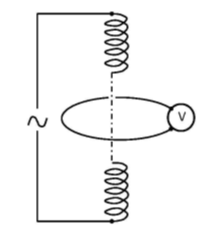
Figure 1. Circuits for the Maxwell-Lodge effect representation [34].
Daibo et al. [36] measured the MLE, using a coiled coil (Figure 2): a very long flexible solenoid whose return-current wire ran through the coil’s center to create a pure vector potential with B = 0. Several secondary coils were passed through the hollow core of the vector-potential coil. The coiled coil (primary) was driven with alternating current that induced voltages in the secondary coils that were path independent and occurred, when enclosed by a (super)conducting material. Daibo [37] patented the novel vector-potential transformer (VPT) and related devices, involving high precision measurements in: living organisms (e.g., medical diagnostics), sea water, nuclear-power-plant reactor pressure vessels, and AC electric-field generation without bare electrodes in corrosive media.
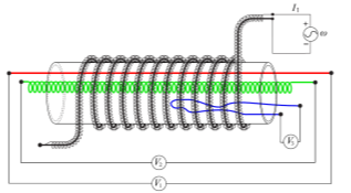
Figure 2. VPT with secondary circuit coil configurations [36].