1. Introduction

Clustering divides a dataset into groups so that points in the same group are more similar to each other than to points in other groups. Classical k-means makes hard assignments: each observation belongs to exactly one cluster. Many real datasets, however, contain points that lie between groups. Examples include mixed pixels in satellite imagery, transitional tissue in medical scans, and customers with mixed purchasing behavior. Hard assignment discards this uncertainty.

Fuzzy k-means addresses this by drawing on fuzzy set theory. Each point receives a membership value between 0 and 1 for every cluster, and its memberships across all clusters sum to 1. Dunn introduced the approach in 1973 as a fuzzy relative of the ISODATA procedure^[1]. Bezdek generalized it in 1981 by introducing an adjustable fuzzification exponent^[21][32]. The names "fuzzy c-means" and "fuzzy k-means" describe the same family of algorithms: Bezdek's notation uses c for the number of clusters, while much of the machine learning literature uses k.

2. Mathematical Formulation

Let A = {u₁, …, u_m} be m data points in ℝ^d, to be grouped into k clusters with centers c₁, …, c_k. Let w_ab be the membership of point u_b in cluster a. FKM minimizes

E_s(C, W; A) = Σ_b=1^m Σ_a=1^k (w_ab)^s ‖u_b − c_a‖², s > 1

subject to

Σ_a=1^k w_ab = 1 for all b; w_ab ∈ [0, 1]; 0 < Σ_b=1^m w_ab < m for all a.

The first constraint makes each point's memberships sum to 1. The last ensures that no cluster is empty and no cluster absorbs every point completely.

The exponent s, often written m in the literature, is the fuzzifier. It controls how soft the partition is. As s approaches 1, memberships approach 0 or 1 and FKM reduces to hard k-means. As s grows large, every membership approaches 1/k and the partition loses its structure. A value of s = 2 is the most common default.

3. Algorithm

The objective has no closed-form minimizer, so FKM uses alternating optimization:

1. Choose the number of clusters k, the fuzzifier s, a stopping tolerance ε, and initial cluster centers.
2. Update the memberships with the centers held fixed:

w_ab = [ Σ_l=1^k ( ‖u_b − c_a‖ / ‖u_b − c_l‖ )^2/(s−1) ]⁻¹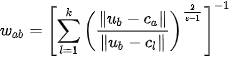

3. Update the centers as membership-weighted means with the memberships held fixed:

c_a = Σ_b=1^m (w_ab)^s u_b / Σ_b=1^m (w_ab)^s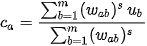

4. Repeat steps 2 and 3 until the largest change in any membership falls below ε.

Each iteration costs O(mkd). Theoretical analyses show that the iterates converge to a local minimizer or a saddle point of the objective^[73][4][85]. In practice, the algorithm is usually run several times from different initializations.

Common initialization strategies include selecting k data points at random as starting centers, initializing the membership matrix with random values that satisfy the constraints, or running hard k-means first and using its centers as the starting point. The stopping tolerance ε is typically set to a small value such as 10⁻³ to 10⁻⁵, often combined with a maximum number of iterations. Once the algorithm converges, a crisp labeling can be obtained when needed by assigning each point to the cluster in which it has the highest membership, a step known as defuzzification.

4. Variants

Standard FKM uses Euclidean distance, which favors roughly spherical clusters of similar size. Many variants change the distance measure or the objective to handle other data geometries:

• Gustafson–Kessel clustering gives each cluster its own covariance matrix, so clusters can take ellipsoidal shapes^[46].
• Possibilistic c-means relaxes the sum-to-one constraint so that outliers receive low membership in every cluster. This reduces their influence on the cluster centers^[57].
• Kernel-based FKM computes distances in a kernel-induced feature space, which helps capture non-linearly separable structure^[108].
• Spatially constrained FKM for image segmentation adds information from neighboring pixels, which makes it more robust to pixel-level noise^[139].
• Divergence-based FKM replaces Euclidean distance with a divergence measure. Banerjee et al. showed that centroid-based clustering extends naturally to the family of Bregman divergences [9]. Karlekar et al. proposed FKM with the S-distance, derived from the S-divergence on positive definite matrices^[1110][141]. They showed that the S-distance is a metric and an f-divergence but not a Bregman divergence, and gave a convergence analysis for the modified algorithm. The S-distance is defined only for strictly positive feature vectors, so it requires positive-valued data or a suitable transformation. Seal et al. studied a related approach using a Jeffreys-divergence-based similarity measure^[1211].

5. Relation to Other Methods

FKM is closely related to two other widely used clustering approaches. Hard k-means is its limiting case: as the fuzzifier approaches 1, the membership update assigns each point entirely to its nearest center, and the center update becomes the ordinary cluster mean.

FKM also resembles Gaussian mixture models (GMMs) fitted with the expectation–maximization (EM) algorithm, since both produce soft assignments. The two differ in how those assignments are defined. In a GMM, each assignment is a posterior probability derived from an explicit probabilistic model of the data, and the algorithm also estimates covariance matrices and mixing proportions. In FKM, memberships come from relative distances to the cluster centers and the fuzzifier, without an underlying density model. As a result, FKM is simpler to implement and has fewer parameters, while GMMs offer a probabilistic interpretation and model elongated or unequal clusters more naturally.

6. Evaluating Fuzzy Partitions

Cluster quality is measured with validity indices. Fuzzy-specific internal indices, such as the partition coefficient and the Xie–Beni index, measure how compact and well separated the fuzzy clusters are without reference to ground truth [2, 6]. General internal indices, such as the silhouette, Dunn, and Davies–Bouldin indices, can be applied after converting memberships into crisp labels. When ground-truth labels are available, external indices such as the adjusted Rand index (ARI) and normalized mutual information (NMI) measure agreement between the clustering and the true classes.

7. Applications

FKM is useful wherever class boundaries are gradual or uncertain. In medical imaging, it separates tissue types in MRI scans, where boundary voxels often contain more than one tissue^[139]. In remote sensing, it supports land-cover classification from multispectral satellite imagery, where a single pixel may cover several surface types^[1110]. In agriculture, it segments crop and leaf images and delineates management zones within fields, where soil and yield properties change gradually rather than at sharp boundaries. It is also used in general pattern recognition, data mining, document organization, and customer segmentation. In each case, graded memberships carry useful information about how uncertain an assignment is.

8. Limitations

FKM has several practical limitations:

• The number of clusters and the fuzzifier must be chosen in advance, and results can be sensitive to both.
• Results depend on initialization, and the algorithm can converge to a poor local minimum.
• Standard FKM is sensitive to outliers, because the sum-to-one constraint forces every point to belong somewhere.
• With Euclidean distance, it favors spherical clusters of comparable size.
• Computing distances to every center at every iteration becomes expensive on very large datasets.

The variants described above each address one or more of these limitations.

References

- Wang Peizhuang; Pattern Recognition with Fuzzy Objective Function Algorithms (James C. Bezdek). SIAMJ. C. Dunn; A Fuzzy Relative of the ISODATA Process and Its Use in Detecting Compact Well-Separated Clusters. J. RCybevrn. 19873, 25, 442-442. [CrossRef], 3, 32-57. [CrossRef]
- James C. Bezdek; Robert Ehrlich; William Full; FCM: The fuzzy c-means clustering algorithm. Comput. Geosci. 1984, 10, 191-203. [CrossRef]Donald E. Gustafson; William C. Kessel. Fuzzy clustering with a fuzzy covariance matrix; Institute of Electrical and Electronics Engineers (IEEE): Piscataway, NJ, United States, 1978; pp. 761-766. [CrossRef]
- Donald E. Gustafson; William C. Kessel. Fuzzy clustering with a fuzzy covariance matrix; Institute of Electrical and Electronics Engineers (IEEE): Piscataway, NJ, United States, 1978; pp. 761-766. [CrossRef]L. Groll; J. Jakel; A New Convergence Proof of Fuzzy c-Means. IEEE Trans. Fuzzy Syst. 2005, 13, 717-720. [CrossRef]
- R. Krishnapuram; J.M. Keller; A possibilistic approach to clustering. IEEE Trans. Fuzzy Syst. 1993, 1, 98-110. [CrossRef]Arindam Banerjee; Srujana Merugu; Inderjit Dhillon; Joydeep Ghosh. Clustering with Bregman Divergences; Society for Industrial & Applied Mathematics (SIAM): Philadelphia, PA, United States, 2004. [CrossRef]
- X.L. Xie; G. Beni; A validity measure for fuzzy clustering. L. Groll; J. Jakel; A New Convergence Proof of Fuzzy c-Means. IEEE Trans. PatternFuzzy Anal. Mach. IntellSyst. 1991, 2005, 13, 841-847. [CrossRef], 717-720. [CrossRef]
- Höppner, F.; Klawonn, F. A contribution to convergence theory of fuzzy c-means and derivatives. . R. Krishnapuram; J.M. Keller; A possibilistic approach to clustering. IEEE Trans. Fuzzy Syst 200. 1993, 11, 682-694., 98-110. [CrossRef]
- L. Groll; J. Jakel; A New Convergence Proof of Fuzzy c-Means. X.L. Xie; G. Beni; A validity measure for fuzzy clustering. IEEE Trans. FuzzyPattern Anal. Mach. SystIntell. 2005, 1991, 13, 717-720. [CrossRef], 841-847. [CrossRef]
- Arindam Banerjee; Srujana Merugu; Inderjit Dhillon; Joydeep Ghosh. Clustering with Bregman Divergences; Society for Industrial & Applied Mathematics (SIAM): Philadelphia, PA, United States, 2004. [CrossRef]Karlekar, A.; Seal, A.; Krejcar, O.; Gonzalo-Martín, C. . Fuzzy k-means using non-linear S-distance. . IEEE Access 2019, 7, 55121–55131.
- 10. Zhang, D.Q.; Chen, S.C. Clustering incomplete data using kernel-based fuzzy c-means algorithm.. Neural Sra S. Positive definite matrices and the S-divergence. Process. LettAm. Math. Soc 2003, 16, 18, 155–162.44, 2787–2797.
- Karlekar, A.; Seal, A.; Krejcar, O.; Gonzalo-Martín, C. . Fuzzy k-means using non-linear S-distance. . IEEESeal, A.; Karlekar, A.; Krejcar, O.; Gonzalo-Martín, C. Fuzzy c-means clustering using Jeffreys-divergence based similarity measure.. Appl. AccessSoft Computing 202019, 7, 55121–55131., 88, 106016.
- Seal, A.; Karlekar, A.; Krejcar, O.; Gonzalo-Martín, C. Fuzzy c-means clustering using Jeffreys-divergence based similarity measure.. Appl. Soft Keh-Shih Chuang; Hong-Long Tzeng; Sharon Chen; Jay Wu; Tzong-Jer Chen; Fuzzy c-means clustering with spatial information for image segmentation. Comput. Med. Imaging Graph. 2020, 88, 106016.6, 30, 9-15. [CrossRef]
- Keh-Shih Chuang; Hong-Long Tzeng; Sharon Chen; Jay Wu; Tzong-Jer Chen; Fuzzy c-means clustering with spatial information for image segmentation. Comput. Med. Imaging Graph. 2006, 30, 9-15. [CrossRef]
- Sra S. Positive definite matrices and the S-divergence. Proc. Am. Math. Soc 2016, 144, 2787–2797.
- J. C. Dunn; A Fuzzy Relative of the ISODATA Process and Its Use in Detecting Compact Well-Separated Clusters. J. Cybern. 1973, 3, 32-57. [CrossRef]