Streamflow is one of the most important hydrologic phenomena, as both its excess and scarcity can lead to floods and droughts—natural disasters that can cause significant damage and even death. This makes it critically important to model, forecast, and synthesize streamflow to understand its behaviour, anticipate extremes, and support effective water resource management. Towards achieving the foregoing challenges, researchers have developed a wide range of models—from simple regression-based techniques to advanced machine learning and deep learning approaches. In this section, the fundamental properties of streamflow are first explored. Following this, a historical overview of streamflow synthesis approaches is presented.
1.1. Understanding the Principles of Streamflow Synthesis
Any phenomenon that undergoes continuous changes over time is considered a process. Hydrologic phenomena, such as precipitation, infiltration, evaporation, and runoff (or streamflow), are dynamic and complex, influenced by natural factors (e.g., climate, topography, vegetation), anthropogenic activities (e.g., land use changes, water extraction, urbanization), and unknown physical interactions. This inherent complexity makes hydrologic phenomena
stochastic rather than deterministic (
[1][2][1,2]).
Moreover, hydrological processes are continuous in nature. However, to measure, study and model these processes effectively, they are treated as discrete, which means that they are discretized into specific time intervals (e.g., hourly, daily, or monthly) for practical reasons. In this context, the discrete time intervals between successive observations make them
a time series [3][4][5][6][3,4,5,6].
In the study of streamflow as a
stochastic time series, the choice of time interval is crucial and can vary between daily, weekly, monthly, or annual observations. This discrete time interval should be determined based on the specific objectives and requirements of the hydrologic project. For example, in the design of drainage structures, the hourly streamflow might be more appropriate, while in long-term water resource management, monthly or annual data can be used. Each of these types of data sets has different behaviour; for instance, annual series tend to lack visible cycles due to aggregation, while monthly series typically show seasonal patterns. Daily streamflow series, in contrast, are characterized by rapid peaks and sharp recessions, reflecting short-term hydrologic dynamics. In general, shorter interval series are more complex and challenging to model, whereas longer interval series (e.g., annual) simplify the modelling and parameter estimation process
[2][7][8][2,7,8].
Hydrologic time series can be categorized as either historical, derived from measurements or observations at specific time intervals, or synthesized, generated with a specific objective of applying them in water resource system planning, design, and operations, commonly referred to as
operational hydrology [2][9][10][2,9,10]. The synthesized realizations carry the information from historical time series and are designed to mimic pre-specified properties derived from historical data
[11][12][11,12].
From a simple perspective, each synthesized realization of streamflow could represent a series of events that occurred before the actual measurements began, since historical data has only been recorded for almost a century, but the hydrologic processes were already at work for thousands of years before the formal recording started. This means that a severe flood recorded in the historical data might not be the worst ever flood that has occurred, and similarly, the worst recorded drought might not be the most extreme
[11][13][14][11,13,14]. The most severe events, those not recorded in the historical data, might still occur in the future. This broader set of possible but unobserved outcomes is referred to as the
population, the full range of potential streamflow values that could arise under the same governing processes.
Mathematically, it can be said that by streamflow synthesis, the ensemble of
m streamflow series would be obtained. If
m → ∞ , characteristics of the population would be estimated, which means that the probability of the ensemble characteristics being equal to the population characteristics will be equal to 1 (
Pr x s a m p l e ≅ X p o p u l a t i o n ≈ 1 )
[2]. More accurately, an available historical sample is synthesized, and more information from the population is obtained. It all depends on the information extracted from the historical streamflow record, as this information defines the pre-specified properties that must be mimicked in the synthesized series. Based on such knowledge, an appropriate model is selected, one that can reproduce the identified properties. As more complex characteristics are recognized, more advanced models are required to capture them effectively.
1.2. What Do We Know About Streamflow Characteristics
Before the 1950s, basic statistical moments, particularly measures of central tendency such as mean or median and dispersion such as variance, skewness and kurtosis, were the only information available. These simple metrics were considered sufficient representations of the underlying hydrologic behaviour.
In the 1950s and the early 1960s, the temporal dependence structure of streamflow became a key focus in hydrologic research. Streamflows were commonly characterized as a first-order Markov process, and the strong autocorrelation at the first (and the second) lag was used to quantify short-term dependence, which needs to be preserved by models designed to synthesize streamflow. The findings by Hurst introduced a new dimension to our understanding of streamflow by revealing the presence of long-term persistence, now known as the Hurst phenomenon.
Hurst
[15] analyzed around 900 annual time series datasets covering various environmental variables like streamflow, precipitation, lake levels, tree rings, and atmospheric pressure. He observed that the adjusted range represented by
R, which is calculated as the difference between the largest excess (
Pn) and the greatest deficiency (
Qn) over a steady flow period of n years, varied with the length of the dataset (denoted by n) according to a specific relationship of
R / S ~ n h , where
R/S is the rescaled range, and
S is the sample standard deviation of the dataset. Hurst estimated a coefficient (
h) through a formula involving
R and
S, providing insights into the long-term storage requirements of the Nile River and other hydrological systems. The coefficient (
h) serves as a direct measure of long-term persistence within a time series of data
[16][17][18][19][16,17,18,19]. A value of 0.5 <
h < 1 indicates a persistent time series, while
h = 0.5 corresponds to a random walk pattern
[20][21][20,21].
The identification of long-term persistence introduced new complexity into the understanding of streamflow behaviour and the broader temporal dynamics of hydrologic processes. Klemeš
[22] argued that the persistence reflected by the Hurst coefficient might not arise from a single identifiable cause. Instead, it could result from a genuinely long-memory physical process (such as large-scale climatic influences), nonstationarity in the data (like gradual shifts in the mean), the effects of storage and release mechanisms in natural or engineered systems (e.g., soils, lakes, or reservoirs), or a combination of these factors, which are often difficult to understand and disentangle in practice due to data limitations and system complexity. This suggests that the memory structure of hydrologic processes is too complex to be fully explained by a single factor, such as the Hurst coefficient, even though it is widely accepted and used by hydrologists as an indicator of long-term persistence
[5][12][16][21][22][23][24][25][26][27][28][29][30][31][32][33][34][35][36][37][5,12,16,21,22,23,24,25,26,27,28,29,30,31,32,33,34,35,36,37].
To quantify how patterns and statistical properties change across different temporal scales, revealing underlying structures that are not easily apparent at a single time resolution, the scaling behaviour of streamflow has been investigated in the literature. Several studies have attempted to analyze the scaling properties and underlying statistics
[38][39][40][41][42][38,39,40,41,42]. The existence of a relationship between scaling behaviour and the Hurst coefficient was first highlighted by Gallant et al.
[43] and by Blöschl and Sivapalan
[44] as both scaling behaviour and the Hurst coefficient describe the concept of memory in a time series.
To quantify the scaling behaviour of a system, it is widely accepted that the Power Spectrum Analysis (PSA) represents a powerful tool to determine the scaling behaviour of time series
[44][45][46][47][48][49][50][44,45,46,47,48,49,50]. In PSA, the power of a signal at various frequencies is plotted on a log-log graph. If the power spectrum follows a form
( 1 / f α ) then it is considered to be indicative of a scaling behaviour with a scaling exponent (or the power-law exponent) of
α [40][48][40,48]. When the scaling exponent, α = 0, a time series is considered to exhibit white noise, characterized by random fluctuations with no correlation (and therefore no memory). In contrast, a scaling exponent in the range 0 < α < 2 corresponds to pink noise. For the scaling exponent, α = 2, the behaviour is identified as brown noise or Brownian motion. Finally, for α > 2, the series represents a black noise.
Koscielny-Bunde et al.
[41] analyzed daily runoff time series from 18 representative rivers in southern Germany and 23 international rivers, and in all cases found that the fluctuations exhibited self-affine scaling behaviour over time scales ranging from weeks to decades. Livina et al.
[28] highlighted that the river flow time series exhibits clear scaling behaviour, characterized by strong short-term correlation and reduced long-term correlation, likely due to aquifer (groundwater) storage effects. Dolgonosov et al.
[45] discussed that spectral slopes vary across different frequency regions, providing evidence of multi-scale dynamics in streamflow behaviour. Thompson and Katul
[49] showed that streamflow exhibits a robust power-law in the scaling behaviour that is largely insensitive to whether the catchment response is modelled linearly or nonlinearly, and to spatial variability in rainfall, provided the rainfall retains its spectral characteristics. They also concluded that multiple hydrologic processes and flow pathways can produce similar spectral exponents, making the mechanistic interpretation of streamflow spectra difficult despite the consistency in observed scaling patterns.
Using the PSA and detrending fluctuation analysis at 11 gauging stations in the Ebro Basin
[48], investigated the scaling properties of monthly streamflow (1950–2005) in Spain and revealed the presence of characteristics of pink noise in data sets. Such an observation suggests two things: first, that the α-H relationship for non-stationary series requires further investigations in hydrology, and second, that the monthly streamflow may exhibit all types of coloured noise
[51]. Studnicka and Panu
[52] developed an approach to the PSA in monthly streamflow, using reported jumps in the literature
[47][48][47,48] as indicators of the existence of seasonal as well as sub-seasonal cycles, inclusive of a fraction of the cycle and revealed that monthly streamflow exhibited all types of coloured noise in 143 hydrometric stations across Ontario.
The presence of noise can distort scaling behaviour across all time scales, but its influence is particularly strong at shorter time scales, such as monthly
[8]. Thus, the non-stationary monthly streamflow should be characterized not only by its scaling properties and memory effects but also by the evolving patterns embedded within the data. The recognition of such patterns, often reflecting seasonal, sub-seasonal, or anthropogenic influences, adds an important dimension to understanding streamflow behaviour. Discussions around patterns as defining characteristics of monthly streamflow date back to the 1960s.
During the 1970s, following the introduction of disaggregation models by Harms and Campbell
[53], monthly streamflow began to be treated as a non-stationary time series due to its strong seasonality and periodicity
[5]. Panu et al.
[54] and Panu and Unny
[55] suggested that recurring patterns, such as cyclicity and seasonality, are inherent features of hydrologic time series. Thus, by treating each seasonal segment as an object and grouping similar objects across years, they emphasized that these patterns not only exist but can also be quantitatively analyzed through pattern recognition techniques.
Moreover, streamflow exhibits two interrelated characteristics: emergent behaviour, shaped by external climatic, geological, and anthropogenic influences, and self-organization, which arises from internal hydrologic feedback such as infiltration, storage, and routing processes. These interacting dynamics contribute to the inherent complexity of streamflows. The dual nature of streamflows can be quantitatively assessed using normalized Shannon entropy. Emergence (E) reflects the degree of unpredictability or information content in a time series, while self-organization (S) is defined as the reduction in this entropy, indicating the underlying structure or order. The product of these two components, scaled by a factor of four, yields a normalized complexity measure (C), which ranges from 0 (complete randomness or total disorder) to 1 (an optimal balance between variability and structure).
Mujumdar and Kumar
[56] have shown that this complexity measure can distinguish streamflow dynamics across different catchment types, such as low- and high-snow-dominated basins, and is significantly associated with persistence, particularly in low-snow regions. Piran and Panu
[57] indicated that while complexity captures a balance between order and unpredictability in streamflows, it is not directly associated with the persistence or memory-retaining nature of the streamflow process in snow-dominated regions of Ontario. Complexity reflects the ability of a system to generate new information while maintaining underlying patterns; however, whether this behaviour stems from external non-deterministic influences, such as climate variability, or it arises from deterministic chaos, remains a subject for further investigation.
While the presence of recurring patterns, such as seasonality, periodicity, and scaling behaviour, reflects a certain degree of regularity in streamflow time series, these patterns coexist with inherent nonlinearities that confound the dynamics of hydrologic systems, particularly at the discharge rates. Streamflows are governed by a complex interplay of climatic, topographic, and land surface processes, all of which can interact in multiple nonlinear ways. As a result, even small differences in initial conditions, such as antecedent soil moisture, rainfall intensity, or vegetation cover, can lead to disproportionately large differences in hydrologic responses. This phenomenon, known as
sensitive dependence on initial conditions, underscores the chaotic nature of streamflows
[8]. Numerous methods have been developed to identify chaos in time series data, with most grounded in the fundamental concept of phase space reconstruction, a technique used to visualize and analyze the underlying dynamics of complex systems
[58][59][60][61][62][58,59,60,61,62].
In the context of non-stationary time series influenced by periodicity, the choice between chaotic modelling approaches and pattern recognition systems is guided by the nature of the data set and the specific modelling objectives. Chaotic approaches are often employed when the underlying dynamics exhibit complex, nonlinear behaviour, whereas pattern recognition systems are typically preferred for detecting and adapting to evolving patterns, especially when the patterns are perceived as simpler or when ease of implementation is prioritized
[63]. Understanding key characteristics of streamflow informs the selection of appropriate modelling approaches. As more aspects of streamflow are quantified, models are increasingly expected to replicate these features.
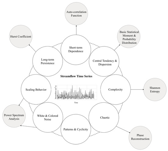
Figure 1 illustrates key known characteristics of streamflows to date, along with the corresponding methods used to quantify them.
Figure 1. Key known characteristics of streamflow (white circles) and the corresponding methods commonly used to quantify each characteristic (grey circles).
1.3. Role of Streamflow Synthesis in Operational Hydrology
Traditionally, water resource engineers have utilized the Rippl mass curve approach, often in combination with historical streamflow data, to estimate the capacity of reservoirs, which can be used either in the construction or maintenance of storage
[64]. The Rippl mass curve is used to analyze and design reservoir storage capacity
[65].
Storage-Yield-Reliability (S-Y-R) equations are used to determine a reservoir capacity S (active storage), required to deliver a desired yield Y, with the expected inflow Q, considering losses L at time t ( S t − 1 + Q t − Y t − L t = S t ). The analysis involves estimating the reservoir capacity to achieve a certain yield with a specified level of reliability or determining the yield from an existing reservoir of known capacity.
The S-Y-R equations can be used in water resource engineering to estimate the reliability of a reservoir system in meeting water supply demands over a specified period (Reliability = N s / N ; where N s is the number of time intervals during which demand was met, and N is the total number of time intervals. Stochastic streamflow models have been recommended to derive the probability distribution of required reservoir capacity for maintaining specified releases. However, estimating parameters of stochastic streamflow models from relatively short hydrological records introduces uncertainty in the derived S-Y-R relationships.
The traditional approaches (deterministic approach) to reservoir analysis faced criticism, leading to a shift towards streamflow synthesis facilitated by the development of stochastic hydrology. This transition to a stochastic approach, in which the aim is to understand how the reservoir system behaves under different scenarios and conditions, such as varying inflow patterns, changing water demand, and operational strategies, requires streamflow synthesis
[23].
Vogel and Stedinger
[64] examined whether estimated storage capacity based on synthetic streamflow sequences, despite their limitations, offers more accurate estimates of required storage capacity volumes compared to those obtained through traditional drought-of-record analyses. Their results show that fitting an AR(1) lognormal model leads to more accurate estimates of annual storage requirements than relying solely on historical flows, even in situations where flows were not generated with an AR(1) lognormal model. However, estimates of storage capacity obtained by fitting stochastic annual streamflow models to 80-year samples can exhibit significant variability. Understanding yield and reliability estimates is crucial within the context of typical reservoir system design applications.