Traumatic brain injury (TBI) affects approximately 250 in 100,000 individuals globally, contributing to 30–50% of trauma-related mortalities, with adolescents, young adults, and the elderly being the most affected groups ^[1][2][1,2]. Mild TBI (mTBI) constitutes 80% of TBI cases, impacting around 42 million people annually, and can result in neuropsychiatric outcomes, impaired functionality, epilepsy, and neurodegenerative diseases ^[3][4][5][6][3,4,5,6]. Despite the rising interest in accurate TBI and mTBI diagnosis through fluid and imaging biomarkers ^[5][7][5,7], limited research has focused on the sole use of computed tomography (CT) or magnetic resonance imaging (MRI) in TBI diagnosis. These modalities are widely accessible yet often demonstrate low sensitivity, especially for mTBI [8].

Recent advancements have witnessed a surge in TBI research utilizing machine learning, aiding in predicting mortality, long-term outcomes, intracranial pressure, and various other clinical parameters ^{[9][10][11][12][13][14][15][16][17][18][19][20][21][22][23][24][25][26][27][28][29][30][31][32][33][34][35][36][37][38][39][40][41][42][43][44][45][46][47][48][49][50][51][52][53][54][55]}[9,10,11,12,13,14,15,16,17,18,19,20,21,22,23,24,25,26,27,28,29,30,31,32,33,34,35,36,37,38,39,40,41,42,43,44,45,46,47,48,49,50,51,52,53,54,55].

2. Machine Learning

Machine learning allows computers to learn from data, training algorithms to recognize patterns and make predictions on new, unseen data ^[56][57][56,57]. The typical workflow includes acquiring a dataset, addressing missing values, normalizing the data, choosing algorithms, selecting features, optimizing to avoid overfitting, and, finally, training, validating, testing, and choosing the optimal model [27]. 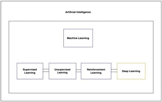There are three primary types of machine learning algorithms: supervised, unsupervised, and reinforcement learning (Figure 1). Supervised learning operates on labeled datasets, while unsupervised learning, which is particularly useful for discovering hidden structures in data, does not require labels. This makes unsupervised learning beneficial, as it sidesteps the often laborious and costly process of data annotation [57]. A specialized subset of machine learning, deep learning, leverages multi-layered artificial neural networks to understand intricate patterns in vast amounts of data. In the context of TBI research, various algorithms have been employed, such as support vector machines (SVMs), artificial neural networks (ANNs), multilayer perceptrons (MPNs), and more. The choice of algorithm often depends on the nature of the data and the desired outcome. While selecting the right algorithm is crucial, choosing pertinent and predictive variables is equally, if not more, vital ^{[10][11][12][13][14][15][16][17][18][19][20][21][22][23][24][25][26][27][28][29][30][31][32][33][34][35][36][37][40][41][42][43][44][46][47][48][49][50][51][52][53][54][55][58][59]}[10,11,12,13,14,15,16,17,18,19,20,21,22,23,24,25,26,27,28,29,30,31,32,33,34,35,36,37,40,41,42,43,44,46,47,48,49,50,51,52,53,54,55,58,59]. Typically, the performance of machine learning models in TBI research is assessed using metrics like sensitivity, specificity, accuracy, and area under the receiver-operating curve (AUROC).

3. Identifying mTBI Using Functional Brain Activity

The difficulty of detecting mTBI through imaging alone has given rise to a substantial body of literature exploring machine learning as a tool for diagnosis, particularly given mTBI’s association with dysregulated neural network functioning [60]. Vergara’s work stands out in this domain. In 2017, Vergara employed dynamic functional network connectivity (dFNC) using fMRI data to differentiate mTBI patients from controls. The ground truth for mTBI diagnosis was based on criteria from the American Congress of Rehabilitation Medicine, which included a Glasgow Coma Scale (GCS) between 13 and 15. They identified four separate dFNC states that a patient could occupy during the five-minute fMRI scan period. Using a linear SVM, participants were classified within each dFNC state into mTBI patients and healthy controls. They were able to achieve a 92% AUROC among 48 patients when classifying using the optimal dFNC state and observed increased dFNC in the cerebellum compared to sensorimotor networks [61]. Another study by the same team in 2016 used resting-state functional network connectivity (rsFNC) from fMRI and fractional anisotropy from diffusion MRI (dMRI), attaining accuracies of 84.1% and 75.5%, respectively, with an SVM model. Increased rsFNC was noted in specific brain regions. Static connectivity, however, as opposed to dFNC, is not able to take into account the dynamic properties of the brain [62]. Later, using SVMs trained with dNFC data on a cohort of 50 mTBI patients, they reported an AUROC of 73% for mTBI prediction [63]. Other researchers have also leveraged fMRI. Luo (2021) used SVMs on resting-state fMRI (rs-fMRI) data to distinguish mTBI from controls among 48 patients, achieving notable diagnostic metrics and focusing on parameters like amplitude of low-frequency fluctuation, degree centrality, and voxel-mirrored homotopic connectivity. By combining multiple such parameters, they were able to distinguish patients with mTBI from controls with an AUROC of 77.8% and accuracy of 81.11% [64]. Fan (2021) and Rangaprakash (2017, 2018) made similar attempts with rs-fMRI and SVM models, yielding accuracies of 0.74 and up to 0.84, respectively ^[63][65][66][63,65,66]. Vedaei et al. concentrated on chronic mTBI, emphasizing its diagnostic significance for guiding treatment. Incorporating rs-fMRI with various metrics in their machine learning approach, they reported AUCs ranging from 80.42 to 93.33% in a study with 100 participants [67].

4. Detecting Axonal Injury with Machine Learning

Several studies have utilized machine learning with diffusor tensor imaging (DTI) metrics to detect axonal injury, which appears to be a key determinant of clinical outcome. Hellyer (2013) and Fagerholm (2016) trained SVM models, focusing on variables like fractional anisotropy and radial diffusivity, to differentiate patients with microbleeds suggestive of axonal injury from controls, achieving sensitivities and specificities often above 0.90. Microbleeds are often considered a surrogate marker of traumatic axonal injury and are visible on gradient-echo and susceptibility-weighted imaging, but patients without microbleeds can still have axonal injury. Both studies extended their initial analyses on microbleed patients to the larger group of non-microbleed patients to show generalizability in predicting cognitive function in the larger group of patients when compared to neuropsychological testing ^[68][69][68,69]. Mitra (2016) utilized RF classifiers focusing on fractional anisotropy features to identify diffuse axonal injury in mTBI patients. Among 325 TBI (mean GCS 13.1) and control participants, they achieved a mean classification accuracy of around 68% and sensitivity of 80% [70]. Stone (2016) employed RF classifiers to segment and quantify white-matter hyperintensities, which have shown prognostic value in TBI, on fluid-attenuated inversion recovery (FLAIR) MRI sequences. They used an RF framework to segment images from 24 patients, achieving an accuracy of 0.68 ^[70][71][70,71]. Other studies by Bai (2020), Cai (2018), Minaee (2017), and Senyukova (2011) employed SVM models with DTI metrics, yielding accuracies ranging from 0.68 to 0.96 ^{[72][73][74][75]}[72,73,74,75]. Abdelrahman (2022) combined SVM with principal component analysis (PCA) on DTI indices to classify 52 total TBI patients and controls, achieving an accuracy of 90.5% and AUC of 0.93 [76]. Machine learning’s potential extends to the clinical management of TBI patients with diffuse axonal injury (DAI). Mohamed (2022) employed a CNN to predict favorable or unfavorable outcomes using the Glasgow Outcome Scale (GOS) from MRIs of 38 patients who sustained moderate or severe TBI with MRI evidence of DAI, achieving a sensitivity of 0.997 and AUROC of 0.917 [77]. Bohyn (2022) applied the FDA-cleared machine learning software icobrain to calculate brain lesion volumes in 20 DAI patients, correlating white-matter volume changes with GOS [78]. Tjerkaski (2022) used an RF model with gradient-echo and susceptibility-weighted imaging to develop a novel MRI-based traumatic axonal injury (TAI) grading system to discern between favorable and unfavorable outcomes, achieving an AUC of 0.72 [39].

5. Predicting TBI with CT

CT remains a primary imaging modality for suspected TBI. The urgency of detecting lesions has spurred interest in machine learning to enhance and expedite diagnosis. Automated image analysis through machine learning can streamline the process, reducing the time and potential variability introduced by manual reviews. Recent studies have showcased the potential of convolutional neural networks (CNNs) in this domain. Monteiro (2020) used CNNs to identify and quantify various types of intracranial hemorrhages, achieving sensitivity and specificity up to 0.8 and 0.9, respectively, for small lesions [79]. Keshavamurthy (2017) and Salehinejad (2021) trained SVM models and generalizable machine learning models, respectively, both demonstrating high accuracies and sensitivities in detecting characteristic TBI lesions on CT ^[80][81][80,81]. Midline shift (MLS) in CT due to space-occupying lesions (typically hematomas from intracranial hemorrhage in TBI patients) is a prognostic factor in TBI. Studies indicate that TBI patients with MLS less than 10 mm have notably better outcomes than those with more significant shifts [82]. Machine learning’s automated MLS measurement can minimize observer variability. Both Nag (2021) and Yan (2022) employed CNNs for MLS estimation, achieving commendable accuracies greater than 85% and consistency across different types of intracranial hemorrhages when compared to hand-drawn MLSs by clinicians across a range of MLS values from a 2 mm cutoff value to greater than 10 mm ^[83][84][83,84]. Predicting long-term outcomes post-TBI can guide critical clinical decisions. Pease (2022) combined a CNN model analyzing CT data with a clinical model to forecast 6-month outcomes in severe TBI. This fusion model outperformed the standard IMPACT model when tested on their internal dataset and even surpassed the predictions of three neurosurgeons [85].

6. Detecting and Quantifying Subdural Hematomas with Machine Learning

Machine learning aids in the segmentation of pathology from normal structures, and in the context of TBI, it offers potential in delineating subdural hematomas (SDHs). Accurate segmentation enables both detection and volumetric analysis. While manual volumetric evaluation can be labor-intensive and is often omitted in clinical practice, machine learning provides a time-efficient alternative. This is vital because SDH volume is crucial for prognosis and surgical intervention considerations and as a predictor of post-operative recurrence ^[86][87][86,87]. Recent endeavors have demonstrated the capabilities of machine learning in this area. Farzaneh (2020) utilized a random forest model to detect and classify the severity of acute SDHs, achieving a sensitivity of 0.99 and specificity of 0.92 [88]. Chen (2022) employed a CNN for volumetric assessment, with the results closely mirroring manual segmentation with an AUROC of 0.83 [89]. Another CNN model designed for comprehensive SDH evaluation, including thickness, volume, and midline shift, showcased a sensitivity of 91.4% and specificity of 96.4% [90]. Chronic SDHs (cSDHs) present unique challenges due to their varied densities and resemblance to brain parenchyma in certain phases [91]. Kellogg (2021) trained CNN models for both pre- and post-operative cSDHs, achieving a DICE score of 0.83 in predicting cSDH volumes [92]. Moreover, insights from a study by Kung et al. highlight the capabilities of machine learning in predicting post-operative recurrence of SDHs by analyzing specific pathological features [93].