Compressive Sensing in Image/Video Compression

Compressive Sensing in Image/Video Compression: Comparison

Please note this is a comparison between Version 1 by Jian Yang and Version 2 by Sirius Huang.

Compressive Sensing (CS) has emerged as a transformative technique in image compression, offering innovative solutions to challenges in efficient signal representation and acquisition.

compressive sensing
sampling
measurement coding
reconstruction algorithm

1. Introduction

In the era of rapid technological advancement, the sheer volume of data generated and exchanged daily has become staggering. This influx of information, from high-resolution images to bandwidth-intensive videos, has posed unprecedented challenges to conventional methods of data transmission and storage. As we grapple with the ever-growing demand for the efficient handling of these vast datasets, a groundbreaking concept emerges—Compressive Sensing [1].

Traditionally, the Nyquist–Shannon sampling theorem [2] has governed our approach to capturing and reconstructing signals, emphasizing the need to sample at twice the rate of the signal’s bandwidth to avoid information loss. However, in the face of escalating data sizes and complexities, this theorem’s practicality is increasingly strained. Compressive Sensing, as a disruptive force, challenges the assumptions of Nyquist–Shannon by advocating for a selective and strategic sampling technique.

In general, CS is a revolutionary signal-processing technique that hinges on the idea that sparse signals can be accurately reconstructed from a significantly reduced set of measurements. The principle of CS involves capturing a compressed version of a signal, enabling efficient data acquisition and transmission. As the Figure 1 shows, in the field of image processing, numerous works have been proposed in each of various domains, exploring innovative techniques and algorithms to harness the potential of compressive imaging ^{[3][4][5][6][7][8][9][10][11]}[3,4,5,6,7,8,9,10,11], efficient communication systems ^{[12][13][14][15][16][17][18][19][20]}[12,13,14,15,16,17,18,19,20], pattern recognition ^{[21][22][23][24][25][26][27][28][29]}[21,22,23,24,25,26,27,28,29], and video processing tasks ^{[30][31][32][33][34][35][36][37][38]}[30,31,32,33,34,35,36,37,38]. The versatility and effectiveness of CS make it a compelling area of study with broad implications across different fields of signal processing and information retrieval.

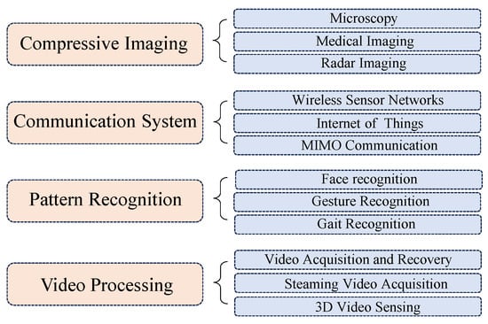
Figure 1.

The applications of compressive sensing in image/video processing.

2. Compressive Sensing Overview

Consider an original signal X, which is an N-length vector that can be sparsely represented as S in a transformed domain using a specific

N \times N

transform matrix

Ψ

, where K-sparse implies that only K elements are non-zero, and the remaining are close to or equal to zero. This relationship is expressed by the equation:

X_{N \times 1 = Ψ_{N \times N S_{N \times 1 .}}}

The sensing matrix, also known as the sampling matrix A, is derived by multiplying an

M \times N

measurement matrix

Φ

by the transform matrix

Ψ

, where

K ≪ M ≪ N

A_{M \times N = Φ_{M \times N Ψ_{N \times N .}}}

The sampling rate, or Compressed Sensing (CS) ratio, denoted as the number of measurements M divided by the signal length N, indicates the fraction of the signal that is sampled:

Sampling Rate (CS ratio) = \frac{M}{N} .

Finally, the measurement vector Y is obtained by multiplying the sensing matrix A with the sparse signal S:

Y_{M \times 1 = Φ_{M \times N Ψ_{N \times N S_{N \times 1 .}}}}

Figure 23 shows the sampling procedure details of CS. The setting and design of the measurement matrix will be elaborated in Section 3.

Figure 23.

Procedure of compressive sensing encoder.

Since the CS reconstruction is an ill-posed problem [39], to obtain a reliable reconstruction, the conventional optimization-based CS methods commonly solve an energy function as:

\hat{X} = arg min X \frac{1}{2} ∥ Φ X - y ∥ 2_{2} + λ R (X),

where

\frac{1}{2} ∥ Φ X - y ∥ 2_{2}

represents the data-fidelity term for modeling the likelihood of degradation, and the

λ R (X)

indicates the prior term with a parameter of regularization of

λ

3. Sampling Algorithms

3.1. Measurement Matrix for Better Reconstructions

One of the fascinating aspects of compressive sensing focuses on the development of measurement matrices. The construction of these matrices is crucial, as they need to meet specific constraints. They should align coherently with the sparsifying matrix to efficiently capture essential information from the initial signal with the least number of projections. On the other hand, the matrix needs to satisfy the restricted isometry property (RIP) to preserve the original signal’s main information in the compression process. However, in the research of ^[40][41][40,41], they verified the possibility that maintaining sparsity levels in a compressive sensing environment does not necessarily require the presence of the RIP, and also demonstrated that it is not a mandatory requirement for adhering to the random model of a signal. Moreover, designing a measurement matrix with low complexity and hardware-friendly characteristics has become more and more crucial in the context of real-time applications and low-power requirements.

In CS-related research a decade ago, random matrices like Gaussian or Bernoulli matrices were often selected as the measurement matrices, which satisfied the RIP conditions of CS. Although these random matrices are easy to implement and contribute to improved reconstruction performance, they come with several notable disadvantages, such as the requirement for significant storage resources and the challenging recovery while dealing with large signal dimensions [42]. Therefore, the issue of the measurement matrix has been widely discussed in recent works.

3.1.1. Conventional Measurement Matrix

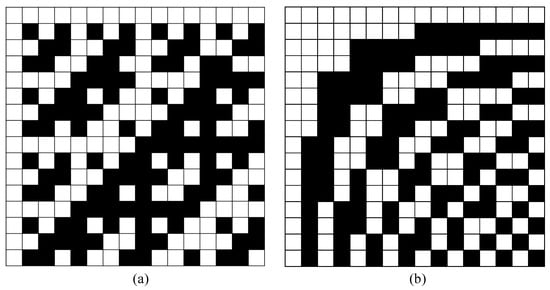
Conventional measurement matrices encompass multiple categories, ranging from random matrices to deterministic matrices, each contributing uniquely to the applications in CS. Random matrices are constructed by randomly selecting elements from a certain probability distribution, such as the random Gaussian matrix (RGM) [43] and random binary matrix (RBM) [44]. The well-known traditional deterministic matrices include the Bernoulli matrix [45], Hadamard matrix [46], Walsh matrix [47], and Toplitz matrix [48]. Figure 34 gives an example of two famous deterministic matrices.

Figure 34.

(

) is Hadamard Matrix and (

) is Walsh Matrix.

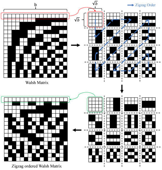
Although these deterministic matrices have been extensively researched and successfully applied to the CS camera, because of their good sensing performance, fast reconstruction, and hardware-friendly properties, they are insupportable when applied to the ultra-low CS ratio [49]. Moreover, for instance, in the work of [44], the information of the pixel domain can be obtained by changing a few rows in the matrix, but the modified matrix results in an unacceptable reconstruction performance, posing enormous challenges for practical applications. In recent years, some studies have been carried out to investigate the effect of Hadamard and Walsh projection order selection on image reconstruction quality by reordering orthogonal matrices ^{[50][51][52][53][54]}[50,51,52,53,54]. A Hadamard-based Russian-doll ordering matrix is proposed in [50], which sorts the projection patterns by increasing the number of zero-crossing components. In the works of ^[51][52][51,52], the authors present a matrix, called the cake-cutting ordering of Hadamard, which can optimally reorder the deterministic Hadamard basis. More recently, the work of [54] designs a novel hardware-friendly matrix named the Zigzag-ordered Walsh (ZoW). Specifically, the ZoW matrix uses the zigzag to reorder the blocks from the Walsh matrix, and, finally, vectored them. The illustration of the process is shown in Figure 45.

Figure 45.

The illustration of the process from Walsh matrix to ZoW matrix.

In the proposed matrix of [54], the low-frequency patterns are in the upper-left corner, and the frequency increases according to the zigzag scan order. Therefore, across different sampling rates, ZoW consistently retains the lowest frequency patterns, which are pivotal for determining the image quality. This allows ZoW to extract features effectively from low to high-frequency components.

3.1.2. Learning-Based Measurement Matrix

Recently, there has been a surge in the development of image CS algorithms based on deep neural networks. These algorithms aim to acquire features from training data to comprehend the underlying representation and subsequently reconstruct test data from their CS measurements. Therefore, some learning-based algorithms are developed to jointly optimize the sampling matrix and the non-linear recovery operator ^{[55][56][57][58][59][60][61]}[55,56,57,58,59,60,61]. Ref. [55]’s first attempt leads into a fully connected layeras the sampling matrix for simultaneous sampling and recovery. In the works of ^[56][57][56,57], the authors present the idea of adopting a convolution layer to mimic the sampling process and utilize all-convolutional networks for CS reconstruction. These methods not only train the sampling and recovery stages jointly but are also non-iterative, leading to a significant reduction in time complexity compared to their optimization-based counterparts. However, only utilizing the fully connected or repetitive convolutional layers for the joint learning of the sampling matrix and recovery operator lacks structural diversity, which can be the bottleneck for a further performance improvement. To address this drawback, Ref. [59] proposes a novel optimization-inspired deep-structured network (OPINE-Net), which includes a data-driven and adaptively learned matrix. Specifically, the measurement matrix

Φ \in R^{M \times N}

is a trainable parameter and is adaptively learned by the training dataset. Two constraints are applied to attain the trained matrix simultaneously. Firstly, the orthogonal constraint is designed into a loss term and then enforced into the total loss, as follows:

L_{orth = \frac{1}{M^{2}} ∥ Φ Φ ⊤ - I ∥ F_{2}}

where I represents the identity matrix. For the binary constraint, they introduce an element-wise operation, defined below:

BinarySign (z) = 1 if z \geq 0 or - 1 if z < 0

Experiments show that their proposed learnable matrix can achieve a superior reconstruction performance with constraint incorporation when compared to conventional measurement matrices.

In general, by learning the features of signals, learning-based measurement matrices can more effectively capture the sparse representation of signals. This personalized adaptability enables learning-based measurement matrices to outperform traditional construction methods in certain scenarios. Another strength of learning-based measurement matrices is their adaptability. By adjusting training data and algorithm parameters, customized measurement matrices can be generated for different types of signals and application scenarios, enhancing the applicability of compressed sensing in diverse tasks. However, obtaining these trainable matrices usually needs a substantial amount of training data and complex algorithms.

3.2. Measurement Matrix for Better Measurement Coding

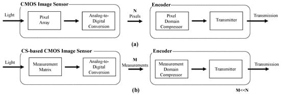
It is noticed that the data reduction from the original signal to CS measurement does not completely equal signal compression, and these measurements can indeed be transmitted directly, but still require a substantial bandwidth. To alleviate the transmitter’s load further, the CS-based CMOS image sensor can collaborate with a compressor to produce a compressed bitstream. However, due to the high complexity, the conventional pixel-based compressor is not suitable for CS systems aiming at reducing the computational complexity and power consumption of the encoder [1]. The difference between conventional image sensors and CS-based sensors is shown in Figure 56.

Figure 56. The illustration of conventional imaging system (a) and CS-based CMOS image sensor (b). The measurement coding is performed on the latter.

Therefore, to further compress measurements, several well-designed measurement matrices for better measurement coding have been recently proposed ^[62][63][62,63]. Wherein, a novel framework for measurement coding is proposed in [63], and designs an adjacent pixels-based measurement matrix (APMM) to obtain measurements of each block, which contains block boundary information as a reference for intra prediction. Specifically, a set of four directional prediction modes is employed to generate prediction candidates for each block, from which the optimal prediction is selected for further processing. The residuals represent the difference between measurements and predictions and undergo quantization and Huffman coding to create a coded bit sequence for transmission. Importantly, each encoding step corresponds to a specific operation in the decoding process, ensuring a coherent and reversible transformation. Extensive experimental results show that [63] can obtain a superior trade-off between the bit-rate and reconstruction quality. Table 1 illustrates the comparison of different introduced measurement matrices that are commonly used in CS.

Table 1.

The PSNR (dB) performance of different matrices on Set5 dataset.

Image	CS Ratio	Measurement Matrices
Image	CS Ratio	RGM [43]	Hadamard [44]	Bernoulli [45]	Toplitz [48]	APMM [63]
Lenna	30%	33.24	28.25	29.87	28.26	33.98
	40%	34.76	29.71	31.24	30.83	36.04
	50%	36.39	30.92	32.48	33.91	37.69
Clown	30%	32.15	24.59	28.36	26.85	32.79
	40%	33.52	26.94	30.49	28.93	35.17
	50%	35.46	28.03	30.67	31.42	37.08
Peppers	30%	33.59	27.78	30.24	30.40	33.83
	40%	34.82	28.03	32.18	32.75	35.50
	50%	36.14	30.17	33.52	33.35	36.74