Research and business today rely heavily on big data and their analysis. However, big data are stored in massive databases that make them difficult to retrieve, analyze, share, and visualize using standard database query tools [1]. For data-driven systems, data exploration is imperative for making real-time decisions and understanding the knowledge contained in the data. However, supporting these systems can be costly, especially regarding big data. One of the most critical challenges posed by big data is the high computational cost associated with data exploration and real-time query processing [2]. To assist with the analysis of big data, several systems have been developed, such as Apache Hive, which typically takes a considerable amount of time to respond to analytical queries [3]. However, approximate results can sometimes be provided for a query in a fraction of the execution time in order to resolve this issue, particularly for aggregation queries. This is because aggregation queries are typically designed to provide a big picture for a large amount of information without having to compute an exact answer [4]. The majority of analytical queries require aggregate answers (such as sum(), avg(), count(), min(), and max()) for a given set of queries (joined or nested queries) over one or more categories (grouped by columns) on a subset (where and the existence of) for big data. Approximate Query Processing (AQP) comes to the rescue by identifying a summary of the population (also known as a synopsis) for discovering trends and aggregate functions [5]. Online aggregations and offline precomputed synopses are the two primary categories that can be used to classify existing AQP approaches. Offline techniques summarize the data distribution and return the approximate results by running queries on these synopses. However, online aggregation techniques progressively generate synopses and return approximate results while data are processing. The traditional approach for both categories uses data distribution to generate a subset of data via statistical methods such as sampling methods [2]. One novel technique for AQP is to take advantage of machine learning to further reduce the execution time, improve accuracy, and support all types of aggregate functions. For instance, the DBEst Query processing engine [6] trains models, notably regression models and density estimators, that provide accurate, efficient, and cost-effective responses to different types of aggregate queries. Learning-based AQP (LAQP) [7] and ML-AQP [8] methods build machine learning models based on historically executed queries. The former builds an error model to predict each incoming query’s sampling-based estimation error, whereas the latter trains models that learn patterns to predict future query results with a bound error by applying prediction intervals constructed using Quantile Regression models. Deep Generative Models (DGMs) are instrumental for approximating complex, high-dimensional probability distributions of data populations [9]. By estimating the probability of each observation, DGMs facilitate the generation of data synopses that faithfully represent underlying distributions. Thirumuruganathan et al. [10] have leveraged DGMs for Approximate Query Processing (AQP) using Variational Autoencoder (VAE). VAE [11] generates new data by encoding input distributions into an interpretable latent space wherein auto-encoders recreate the data. Researchers introduce a novel approach by employing the Generative Adversarial Network (GAN), another state-of-the-art algorithm, for AQP. Unlike VAE, GAN follows a direct implicit density model, allowing it to sample directly from the model’s provided distribution [12] without the need for explicit estimation of the data distribution [13]. This fundamental difference in methodology positions GANs as a more suitable option for AQP in certain contexts. 

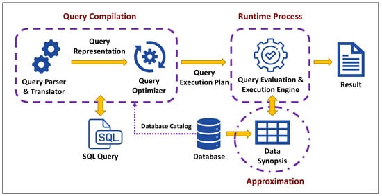
Query processing refers to the process of the compilation and execution of a database query using a specific query language, such as SQL, in order to obtain an approximate result of the requested query. Initially, the query parser validates the query to ensure that the query has been properly stated. Afterward, the query optimizer adjusts the plan to provide a more effective query execution plan. Finally, the query evaluation and execution engine executes the query on the database and returns the results [14]. A traditional database system performs aggregate operations in batch mode, for which a query is submitted and the system processes a huge amount of data slowly and then returns the final result [4]. As a result, the primary concern for query processing is how to process queries efficiently based on computational resources and time. Occasionally, it is impossible to provide exact results in a reasonable amount of time, and an approximate answer with some error guarantee would greatly assist users. In order to approximate a query plan outcome for complex joint queries, the optimizer requires accurate estimates of the sizes of results generated at accurate selectivity estimates. As a result, data synopses can be used to estimate the number of results generated by a query by estimating the underlying data distribution [15].

Approximate Query Processing (AQP) is a method that returns approximations of aggregate query answers using a data synopsis that closely replicates the actual data’s behavior [16]. As a higher level of abstraction, AQP aims to calculate an answer that is approximate to the actual query result based on a data synopsis as a highly compressed and lossy version of the database [17]. In Figure 1, the different phases of query processing are shown, as the query in AQP is executed based on a data synopsis rather than actual data.

Based on a cost-effective approach, approximation accuracy (consequently completion time) is determined by the size of data synopses, which means how much smaller the synopses are than the original database [16]. We can create these synopses using either offline or online techniques. Offline synopses are built using existing data statistics and help answer queries quickly but can involve more complex and resource-intensive methods. With offline methods, database optimization techniques like replication and indexing can be employed to refine the synopsis when the database changes [18]. On the other hand, online synopses allow for real-time query monitoring: giving users preliminary results that are refined as more data are processed and stopping once the results reach a satisfactory level of accuracy and confidence [4].

By taking an online approach, there is no need to make any a priori assumptions. In contrast to the offline approach, creating good data synopses is much more difficult [18]. The Online Analytical Processing (OLAP) system is an example of these systems, and one of its key issues is the regular updating of aggregates to ensure that approximated answers are smooth and continuously improving. By constructing a concise and accurate synopsis of the underlying data distribution, the system consistently strives to reduce the amount of time it takes to complete the task [2].

There may be considerable differences in the structure of the synopsis, and it should be tailored to the problem being addressed. As an example, the AQP synopsis structure is likely to differ from data mining tasks such as change detection and classification [19]. AQP systems should generate an effective synopsis that can be applied to various data distributions and data types within different databases. It is common for big data to produce massive amounts of complex data in a streaming manner. Traditionally, streaming algorithms are evaluated based on three factors: running time, memory complexity, and approximation ratio [20]. Synopsis construction in data streams can be achieved using a variety of techniques:

Sampling methods: It has been demonstrated that sampling is a simple and effective method of obtaining approximate results that provide an error guarantee when compared with other approximate query processing techniques. It is possible to divide a sampling estimation roughly into two stages. Initially, a suitable sampling method must be identified to construct a sampling synopsis from the original dataset, and then a sampling estimator must be analyzed in order to determine its distribution characteristics [21].

Histograms: In the histogram approach, the value range of attributes is divided into K buckets with equal widths, and then the numbers of values falling within each bucket are counted [22]. Based on these statistics, the histogram can then be used to reconstruct the value of the entire dataset within each bucket using the most representative statistics for each bucket [2]. In real-world applications, multiple visits to a data stream can improve accuracy and performance, but this is not realistic. For this reason, one-pass and high-accuracy algorithms are required in order to generate data synopses [21]. A histogram is cheap to compute since only one pass through the relationship is required, but its precision is not always satisfactory [22].

Wavelets: In synopsis construction, wavelets, derived from wavelet transformations in signal processing, play a crucial role. These transformations decompose a function into a set of wavelets using a wavelet decomposition tree, enabling multi-scale and multi-resolution analysis. This unique feature allows wavelets to represent data at various levels of granularity and resolution, making them particularly useful for abstracting and compressing data. To generate a synopsis, the original data are decomposed n times, leveraging the approximation coefficient at each level of the tree to reach an increasingly abstract representation of the data [23]. While conceptually similar to data bucketing in histograms, wavelets differ significantly in their approach. They transform data to compress their most expressive features, a process that is computationally intensive but offers a more nuanced representation. In contrast, histograms generate buckets by analyzing a subset of the original data, which is less computationally demanding but also less detailed at capturing data variations [2].

Sketches: Sketches are a type of probabilistic data structure based on the frequencies of unique items in a dataset [24]. In order to construct the synopses, k random vectors can be selected, and the data can be transformed by dot product to those vectors [19].

Although this section introduced the basic methods for constructing synopses, many other techniques, such as clustering [19] and materialized views [25], can also be used to generate them. Traditional methods have many challenges relating to data type, structure, distribution, and query aggregation functions. Furthermore, synopses provide the most accurate summary using the entire data stream, and it would be inconvenient to retrieve the entire dataset in real-time databases as it changes over time. A discussion of the challenges associated with generating data synopses in relational databases will be presented in the following subsection.

GANs were introduced in computer vision, where they are commonly used to process image data via Convolutional Neural Networks (CNNs). However, they are capable of generating tabular data as well. The GAN architecture has undergone numerous enhancements in recent years as a result of improvement to the architecture among the research community over the past few years [26]. To determine whether or not GAN is an appropriate option for synopsis generation, thfis sectionrst we provides a detailed description of the GAN method and its architecture.

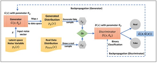
Generative Adversarial Networks are characterized by two neural networks: the generator, which creates data that are intended to mimic the true data distribution, and the discriminator, which evaluates the data to distinguish between the generator’s fake data and the real data from the actual distribution [27]. The generator draws a random vector z from the latent space with the distribution 𝑝𝑧(𝑧). The generator 𝐺(𝑧;𝜃𝑔) then uses a parameter 𝜃𝑔 to map z from the latent space to the data space. Therefore, 𝑝𝑔(𝑥) (the probability density function over the generated data) is used by 𝐺(𝑧) to generate 𝑥𝑔. Then, the discriminator neural network 𝐷(𝑥;𝜃𝑑) receives randomly either 𝑥𝑔 (the generated sample) or 𝑥𝑑𝑎𝑡𝑎 (the actual sample) from the probability density function over the data space 𝑝𝑑𝑎𝑡𝑎(𝑥). The discriminator neural network 𝐷(𝑥;𝜃𝑑) is a binary classification model in which 𝐷(𝑥) returns the probability that x is derived from real data. Therefore, the output of this function is a single scalar that indicates if the passed sample is real or fake. Figure 2 depicts the described process and GAN architecture. The variables 𝜃𝑔 and 𝜃𝑑 are the weights of the generator and discriminator that are learned through the optimization procedure during training.

The goal of the discriminator in training is to maximize the probability that a given training example or generated sample is assigned the proper label, whereas the goal of the generator is to minimize the probability that the discriminator detects real data. Therefore, the objective function can be expressed as a minimax value function, 𝑉(𝐺,𝐷), which is jointly dependent on the generator and the discriminator, where:

The discriminator performs binary classification, which gives a value of 1 to real samples (𝑥∼𝑝𝑑𝑎𝑡𝑎(𝑥)) and a value of 0 to generated samples (𝑧∼𝑝𝑧(𝑧)). Therefore, in the optimal adversarial networks, 𝑝𝑔 converges to 𝑝𝑑𝑎𝑡𝑎 and the algorithm is stopped at 𝐷(𝑥)=1/2, which means the global optimum occurs when 𝑝𝑔=𝑝𝑑𝑎𝑡𝑎 [27].

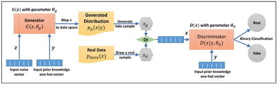
The generation of data in an unconditioned GAN is completely unmanageable in a multimodal distribution. Mirza and Osindero [28] introduced a conditional version of GAN that can provide generators with prior information so that they can control the generation process for different modes. Achieving this objective requires conditioning the generator and discriminator on some additional information, y, where y can be anything from class labels to information about the distribution of data (modes). This can be done by giving the discriminator and the generator Y as an extra input layer in the form of a one-hot vector. In fact, the input noise 𝑝𝑧(𝑧) to the generator is not truly random if the information y is added to it, and the discriminator does not only regulate the similarity between real and generated data but also the correlation between the generated data and input information y. Therefore, the objective function in Equation (1) can be rewritten as follows:

Figure 3 illustrates the structure of a CGAN and how the input information is applied during the process. A majority of applications for conditional GAN are concerned with synthesizing images by giving the label for the image that should be generated. Nonetheless, in the case of tabular data, this could be the shape of data on a multimodal distribution and can be used to inject information as prior knowledge to the generator.

To date, all proposed solutions have been published with the aim of adhering to real data privacy regulations and preventing data leakage during data sharing or for the generation of synthetic data for data imputation and augmentation. By contrast, in AQP applications, it is necessary to generate realistic data rather than synthetic data that is as close to real data as possible. The challenges associated with generating tabular data using GAN have been addressed in a few publications since 2017. The purpose of this section is to introduce promising variants of GAN for tabular data generation, followed by a classification of the proposed solutions based on the previously discussed synopsis construction challenges.

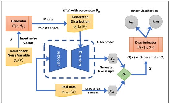
Choi et al. [29] proposed the medical Generative Adversarial Network (medGAN) to generate realistic synthetic patient records based on real data as inputs to protect patient confidentiality to a significant extent. The medGAN generates high-dimensional, multi-label discrete variables by combining an autoencoder with a feedforward network, batch normalization and shortcut connections. With an autoencoder, flow gradients are able to end-to-end fine-tune the system from the discriminator to the decoder for discrete patient records. The medGAN architecture uses MSE loss for numerical columns, cross-entropy loss for binary columns, and the ReLU activation function for both the encoder and decoder networks. The medGAN uses a pre-trained autoencoder to generate distributed representations of patient records rather than directly generating patient records. In addition, it provides a simple and efficient method to deal with mode collapse when generating discrete outputs using minibatch averaging.

Figure 4 shows the medGAN architecture and defines the autoencoder’s role in the training process.

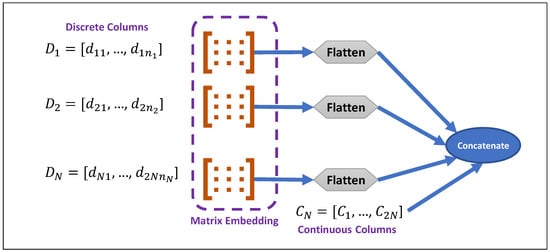
The generator cannot generate discrete data because it must be differentiable. To address this issue, Mottini et al. [30] proposed a method for generating realistic synthetic Passenger Name Records (PNRs) using Cramer GAN, categorical feature embedding, and a Cross-Net architecture for the handling of this issue (categorical or numerical null values). As opposed to simply embedding the most probable category, they used the weighted average of the embedded representation of each discrete category. The embedding layer is shared by the generator and discriminator, resulting in a fully differentiable process as a result of this continuous relaxation. For handling null values, they are substituted with a new category in categorical columns. However, continuous columns fill null values with a random value from the same column and then a new binary column is inserted with 1 for filled rows and 0 otherwise. These additional binary columns are encoded like category columns. It should be noted that in this architecture, both the generator and discriminator consist of fully connected layers and cross-layers. Also, except for the last layer (sigmoid), all layers of the generator use leaky ReLU activations for numerical features and softmax for categorical features. However, the discriminator uses leaky ReLU activations in all but the last layer (linear). Neither batch normalization nor dropout are used in this architecture as in the Wasserstein and Cramer GAN [31]. Data pre-possessing in this algorithm is depicted in Figure 5.

As indicated, discrete values will be embedded using the embedding matrix; then, they will be concatenated with continuous columns of input data.

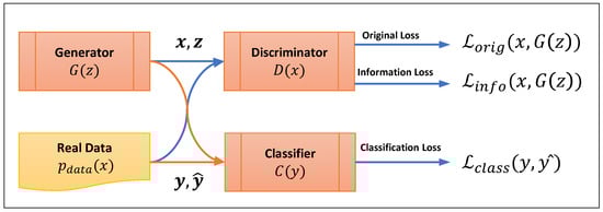
Table-GAN [32] uses GAN to create fake tables that are statistically similar to the original tables but are resistant to re-identification attacks and can be shared without exposing private information. Table-GAN supports both discrete and continuous columns and is based on Deep Convolutional GAN (DCGAN) [33]. Besides the generator and discriminator with multilayer convolutional and deconvolutional layers, the table-GAN architecture also includes a classifier neural network with the same architecture as the discriminator. However, it is trained using ground-truth labels from the original table to increase the semantic integrity of the generated records. Information loss and classification loss are two additional types of loss introduced during the backpropagation process. These functions serve a critical role in balancing privacy and usability while also ensuring the semantic integrity of real and generated data. Information loss functions by comparing the mean and standard deviation of real and generated data. This comparison aims to measure the discrepancy between them. It determines whether they possess statistically similar features from the perspective of the discriminator. On the other hand, classification loss measures the disparity in labeling. It assesses the difference between the actual label of a record and how the classifier predicts it should be labeled. Figure 6 is a representation of the loss functions in the table-GAN architecture.

Xu and Veeramachaneni developed TGAN [34], which is a synthetic tabular data generator for data augmentation that can take into account mixed data types (continuous and categorical). TGAN generates tabular data column-by-column using a Long Short-Term Memory (LSTM) network with attention. The LSTM generates each continuous column from the input noise in two steps. First, it generates a probability that the column comes from mode m, and then, it normalizes the column value based on this probability. TGAN penalizes the original loss function of a GAN by incorporating two Kullback–Leibler (KL) divergence terms. These terms measure the divergence between generated and real data for continuous and categorical columns separately [35]. Therefore, the generator is optimized as follow:

where 𝑢′𝑖 and 𝑢𝑖 are probability distributions over continuous column 𝑐𝑖 for generated and real data, respectively, 𝑑′𝑖 and 𝑑𝑖 are the probability distributions over categorical column 𝑑𝑖 using the softmax function for generated and real data, respectively, 𝑁𝑐 is the number of continuous columns, and 𝑁𝑑 is the number of categorical columns. The authors also proposed a conditional version of TGAN, named CTGAN [36], for addressing data imbalances and multimodal distribution problems by designing a conditional generator with training by a sampling strategy to validate the generator output by estimating the distance between the conditional distributions over generated and real data.

CTAB-GAN [37] was introduced with the ability to encode a mixed data type and a skewed distribution of the input data table; it utilizes a conditional generator, information and classification loss functions derived from table-GAN, as well as CNNs for both the generator and discriminator functions. Since CNNs are effective at capturing the relationships between pixels within an image, therefore, they can be employed to enhance the semantic integrity of created data. However, in order to prepare data tables for feeding the CNN, rows are transformed into the nearest square 𝑑×𝑑 matrix, where $d=Ceil(\sqrt{N_c+N_d\sqrt{})}$ , 𝑁𝑐 and 𝑁𝑑 are the number of continuous and categorical columns, respectively, in a row of the data table, and then, the extra cells values (𝑑×𝑑−(𝑁𝑐+𝑁𝑑)) are padded with zeros.

It is difficult for GAN to control the generation process of data-driven systems; therefore, integrating prior knowledge about data relationships and constraints can assist the generator in generating synopses that are realistic and meaningful. In order to implement this, DATGAN [38] incorporates expert knowledge into the GAN generator by matching the generator structure to the underlying data structure using a Directed Acyclic Graph (DAG). Using DAG, the nodes represent the columns of a data table, while the directed links between them allow the generator to determine the relationship between variables so that one column’s generation influences another. This means if two variables have no common ancestors, they will not be correlated in the generated dataset. In relational databases, there is no particular order in which columns appear in data tables. Nevertheless, the DAG enables data tables to have a specific column order based on their semantic relationship.

GAN has made significant progress in recent years, which has led to the development of novel variants that improve previously introduced versions that had promising results prior to their introduction. Table 1 provides a summary of the variants of GAN that have been discussed herein and highlights the specific architectural advancements and loss functions that have been employed to enhance the performance of each variant. MedGAN, for example, aims to generate high-dimensional discrete columns while avoiding the common pitfall of mode collapse by leveraging an autoencoder network alongside a Feedforward Neural Network (FNN) for generation and a Fully Convolutional Network (FCN) for discrimination. PNR-GAN addresses the challenge of null values in data tables by employing a cross-layer FCN for both the generator and discriminator and utilizes Cramer loss to measure discrepancies. Table-GAN and CTAB-GAN employ Convolutional Neural Networks (CNNs) in their generators to capture the spatial hierarchy of features within tabular data, with CTAB-GAN incorporating conditions from CGAN and AC-GAN for more-targeted data synthesis. CTGAN also adopts this conditional approach but further refines the model to handle non-Gaussian and multimodal distributions effectively by utilizing Wasserstein loss with a gradient penalty for a more stable training process. On the other hand, TGAN and DATGAN leverage Long Short-Term Memory (LSTM) networks in their generators to capture temporal dependencies and correlations within data: a crucial aspect for maintaining integrity when generating sequential or time-series data. These models demonstrate the ongoing refinement of GANs for complex data structures, where the goal is not only to generate new data but to do so with an acute awareness of the inherent relationships within the original dataset.

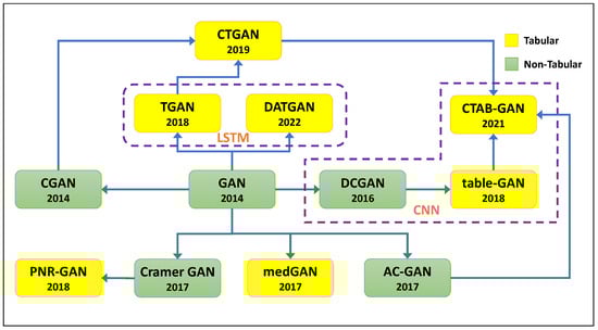
Figure 7 provides a visual representation of the progression and diversification of GAN architectures as they have been specialized for tabular data generation. The diagram traces the lineage of various GAN models starting with the inception of the original GAN framework in 2014. It distinguishes between architectures developed for non-tabular data (in green) and those specifically tailored for tabular data (in yellow), underscoring how foundational models have been adapted and extended to meet the unique challenges of tabular datasets. The evolutionary trajectory begins with the general-purpose GAN and branches into models like DCGAN, which introduced convolutional layers for improved performance on image data. From there, tabular-specific adaptations emerge and innovations continue with the integration of LSTM in TGAN and DATGAN to capture the sequential relationships within data and conditional mechanisms in CTGAN and CTAB-GAN for generating data with given constraints. The figure encapsulates the dynamic and branching nature of GAN development and highlights the critical adaptations made to leverage the power of GANs in the realm of structured data synthesis.