Your browser does not fully support modern features. Please upgrade for a smoother experience.
Please note this is a comparison between Version 2 by Peter Tang and Version 1 by Deyu Tong.
In order to safeguard image copyrights, zero-watermarking technology extracts robust features and generates watermarks without altering the original image. Traditional zero-watermarking methods rely on handcrafted feature descriptors to enhance their performance.
- zero-watermarking
- deep learning
- robustness
- discriminability
1. Introduction
In contrast to cryptography, which primarily focuses on ensuring message confidentiality, digital watermarking places greater emphasis on copyright protection and tracing [1,2][1][2]. Classical watermarking involves the covert embedding of a watermark (a sequence of data) within media files, allowing for the extraction of this watermark even after data distribution or manipulation, enabling the identification of data sources or copyright ownership [3]. However, this embedding process necessarily involves modifications to the host data, which can result in some degree of degradation to data quality and integrity. In response to the demand for high fidelity and zero tolerance for data loss, classical watermarking has been supplanted by zero-watermarking. Zero-watermarking focuses on extracting robust features and their fusion with copyright information [4,5][4][5]. Notably, a key characteristic of zero-watermarking lies in the generation or construction of the zero-watermark itself, as opposed to its embedding.
Commonly, zero-watermarking algorithms are traditionally reliant on handcrafted features and typically involve a three-stage process. The first stage entails computing robust features, followed by converting these features into a numerical sequence in the second stage. The third stage involves fusing the numerical sequence with copyright identifiers, resulting in the generation of a zero-watermark without any modifications to the original data. Notably, the specific steps and features in these three stages are intricately designed by experts or scholars, thereby rendering the performance of the algorithm contingent upon expert knowledge. Moreover, once a zero-watermarking algorithm is established, continuous optimization becomes challenging, representing a limitation inherent in handcrafted approaches.
Introducing deep learning technology is a natural progression to overcome the reliance on expert knowledge and achieve greater optimization in zero-watermarking algorithms. Deep learning has recently ushered in significant transformations in computer vision and various other research domains [6,7,8,9][6][7][8][9]. Numerous tasks, including image matching, scene classification, and semantic segmentation, have exhibited remarkable improvements when contrasted with classical methods [10,11,12,13,14][10][11][12][13][14]. The defining feature of deep learning is its capacity to replace handcrafted methods reliant on expert knowledge with Artificial Neural Networks (ANNs). Through training ANNs with ample samples, these networks can effectively capture the intrinsic relationships among the samples and model the associations between inputs and outputs. Inspired by this paradigm shift, the zero-watermarking method can also transition towards an end-to-end mode with the support of ANNs, eliminating the need for handcrafted features.
2. Zero-Watermarking
The concept of zero-watermarking in image processing was originally introduced by Wen et al. [15]. This technology has garnered significant attention and research interest due to its unique characteristic of preserving the integrity of media data without any modifications. Taking images as an example, the zero-watermarking process can be broadly divided into three stages. The first stage involves the computation of robust features. In this phase, various handcrafted features such as Discrete Cosine Transform (DCT) [16,17][16][17], Discrete Wavelet Transform (DWT) [18], Lifting Wavelet Transform [19], Harmonic Transform [5], and Fast Quaternion Generic Polar Complex Exponential Transform (FQGPCET) [20] are calculated and utilized to represent the stable features of the host image. The second stage focuses on the numerical conversion of these features into a numerical sequence. Mathematical transformations such as Principal Component Analysis (PCA) and Singular Value Decomposition (SVD) are employed to filter out minor components and extract major features [16,21][16][21]. The resulting feature sequence from this stage serves as a condensed identifier of the original image. However, this sequence alone cannot serve as the final watermark since it lacks any copyright-related information. Hence, the third stage involves the fusion of the feature sequence with copyright identifiers. Copyright identifiers can encompass the owner’s signature image, organization logos, text, fingerprints, or any digitized media. To ensure the zero-watermark cannot be forged or unlawfully generated, cryptographic methods such as Advanced Encryption Standard (AES) or Arnold Transformation [22] are often utilized to encrypt the copyright identifier and feature sequence. The final combination can be as straightforward as XOR operations [16]. Consequently, the zero-watermark is generated and can be registered with the Intellectual Property Rights (IPR) agency. Additionally, copyright verification is a straightforward process involving the regeneration of the feature sequence and its comparison with the registered zero-watermark. The process of zero-watermarking technology is illustrated in Figure 1.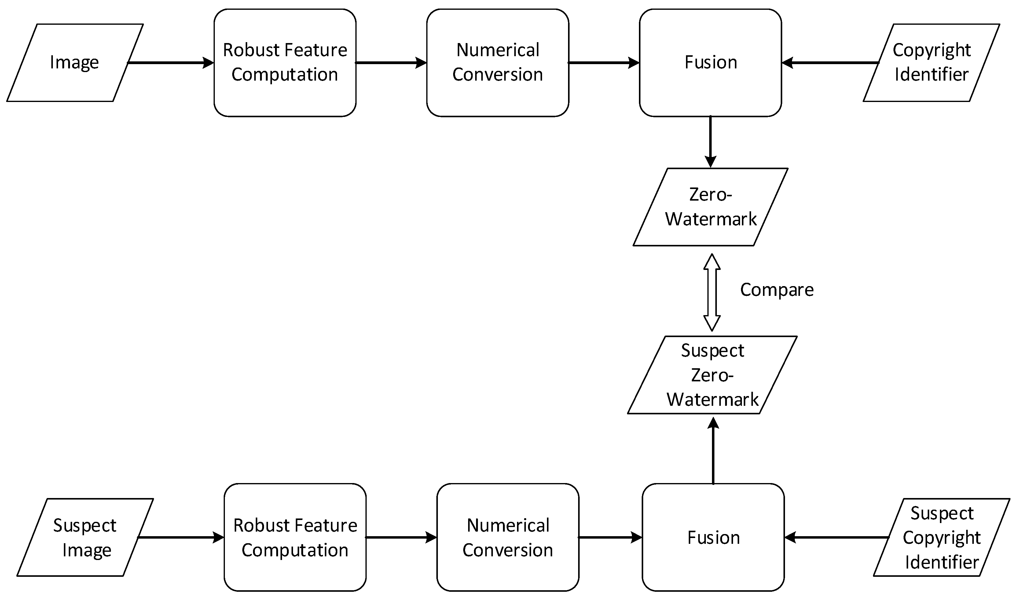
Figure 1.
The process of zero-watermark generation and verification.
3. ConvNeXt
Convolutional Neural Networks (CNN) have been employed as the feature extraction component in existing watermarking methods. However, it is noteworthy that the performance of CNN has become outdated in various tasks. Hence, Liu et al. introduced ConvNeXt, a nomenclature devised to distinguish it from traditional Convolutional Networks (ConvNets) while signifying the next evolution in ConvNets [32]. Rather than presenting an entirely new architectural paradigm, ConvNeXt draws inspiration from the ideas and optimizations put forth in the Swin Transformer [33] and applies similar strategies to enhance a standard ResNet [8]. These optimization strategies can be summarized as follows: (1) Modification of stage compute ratio: ConvNeXt adjusts the number of blocks within each stage from (3, 4, 6, 3) to (3, 3, 9, 3). (2) Replacement of the stem cell: The introduction of a patchify layer achieved through non-overlapping 4 × 4 convolutions. (3) Utilization of grouped and depthwise convolutions. (4) Inverted Bottleneck design: This approach involves having the hidden layer dimension significantly larger than that of the input. (5) Incorporation of large convolutional kernels (7 × 7) and depthwise convolution layers within each block. (6) Micro-level optimizations: These include the replacement of ReLU with GELU, fewer activation functions, reduced use of normalization layers, the substitution of Batch Normalization with Layer Normalization, and the implementation of separate downsampling layers. Remarkably, the amalgamation of these strategies results in ConvNeXt achieving a state-of-the-art level of performance in image classification, all without requiring substantial changes to the network’s underlying structure. Furthermore, a key feature of this preseaper rch lies in its detailed presentation of how each optimization incrementally enhances performance, effectively encapsulated in Figure 2.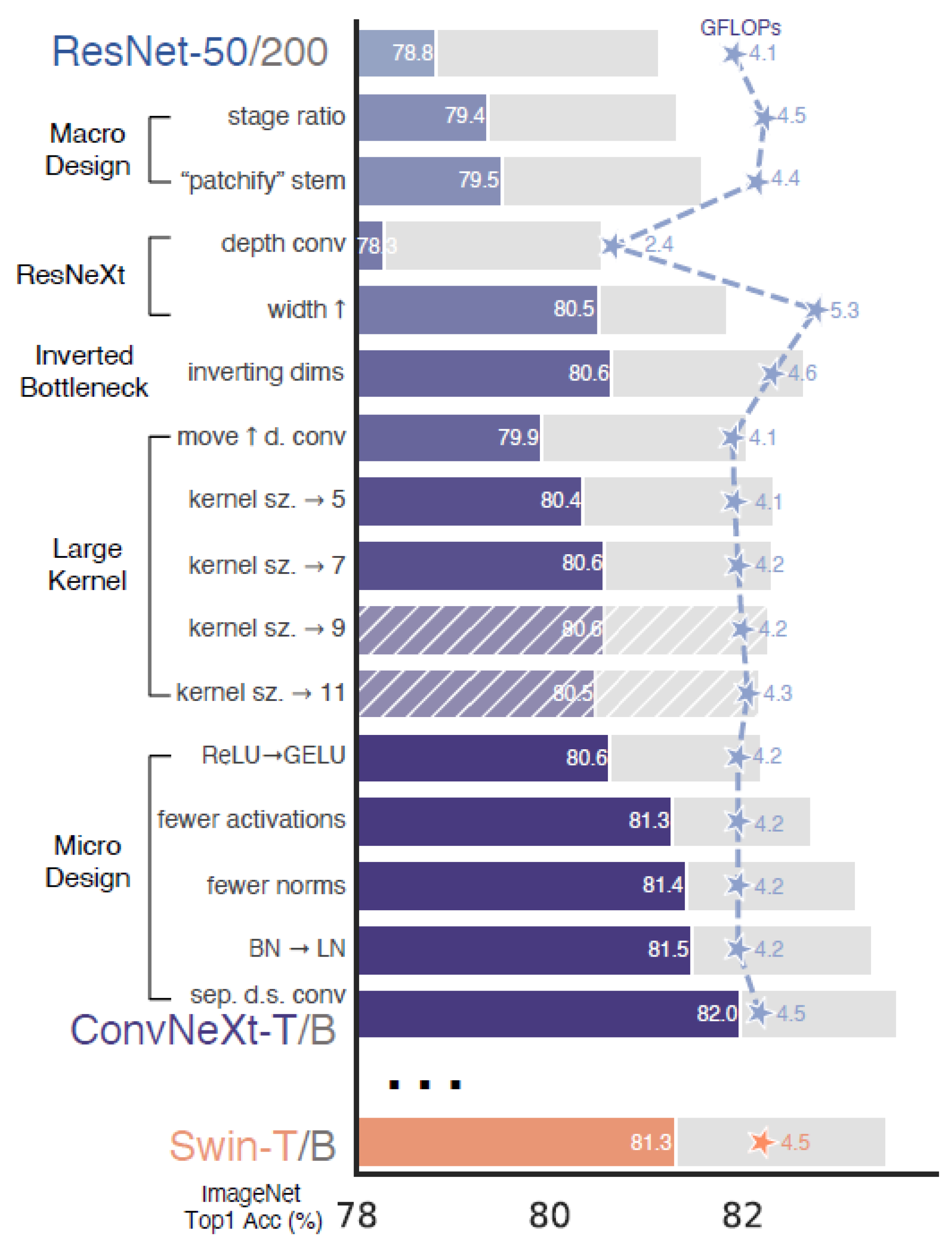
Figure 2. Incremental improvement through optimization steps in ConvNeXt [32]. The foreground bars represent results from ResNet-50/Swin-T, while the gray bars represent results from ResNet-200/Swin-B.
4. LK-PAN
While ConvNeXt offers a straight-line structure that effectively captures local features, it may fall short in dedicating sufficient attention to the global context. To address this limitation and enhance the capabilities of ConvNeXt, a path aggregation mechanism, LK-PAN, is introduced. LK-PAN originates from the Path Aggregation Network (PANet), which was initially introduced in the context of instance segmentation to bolster the hierarchy of feature extraction networks. The primary structure of PANet is depicted in Figure 3.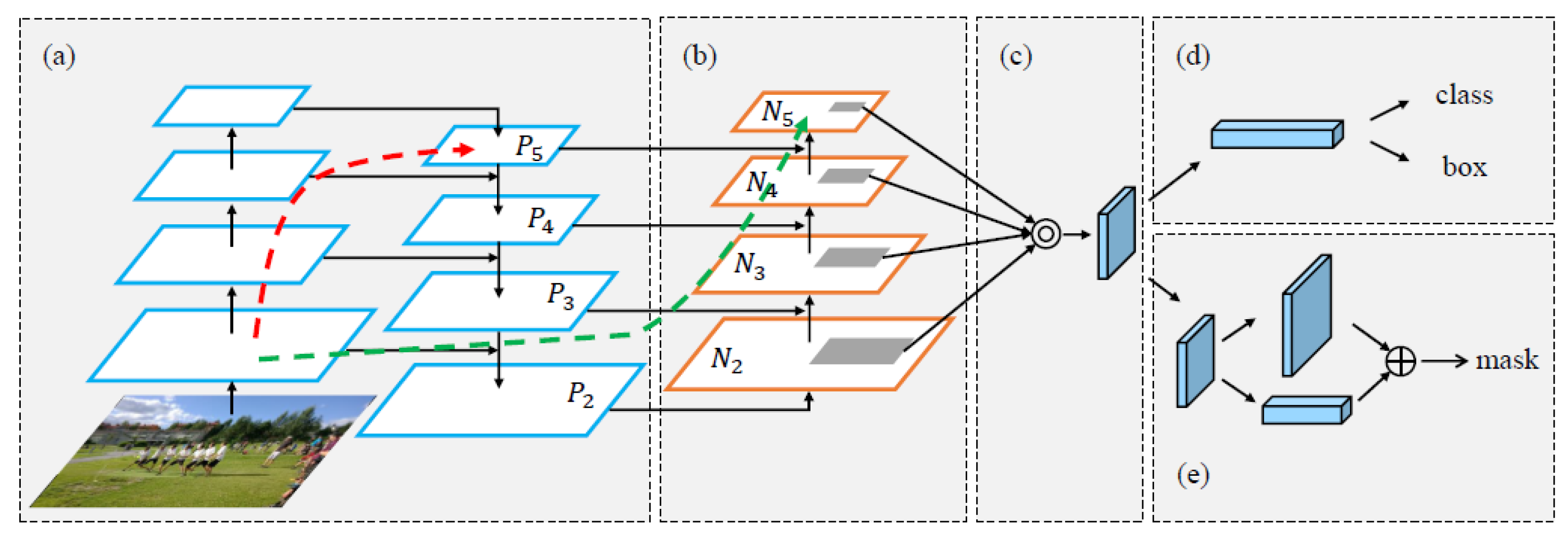
Figure 3. The primary structure of PANet [34]. (a) The backbone part of PANet; (b) Bottom-up path augmentation; (c) Adaptive feature pooling; (d) Box branch; (e) Fully-connected fusion.
References
- Costa, G.; Degano, P.; Galletta, L.; Soderi, S. Formally verifying security protocols built on watermarking and jamming. Comput. Secur. 2023, 128, 103133.
- Razaq, A.; Alhamzi, G.; Abbas, S.; Ahmsad, M.; Razzaque, A. Secure communication through reliable S-box design: A proposed approach using coset graphs and matrix operations. Heliyon 2023, 9, e15902.
- Tao, H.; Chongmin, L.; Zain, J.M.; Abdalla, A.N. Robust Image Watermarking Theories and Techniques: A Review. J. Appl. Res. Technol. 2014, 12, 122–138.
- Liu, X.; Wang, Y.; Sun, Z.; Wang, L.; Zhao, R.; Zhu, Y.; Zou, B.; Zhao, Y.; Fang, H. Robust and discriminative zero-watermark scheme based on invariant features and similarity-based retrieval to protect large-scale DIBR 3D videos. Inf. Sci. 2021, 542, 263–285.
- Xia, Z.; Wang, X.; Han, B.; Li, Q.; Wang, X.; Wang, C.; Zhao, T. Color image triple zero-watermarking using decimal-order polar harmonic transforms and chaotic system. Signal Process. 2021, 180, 107864.
- LeCun, Y.; Bengio, Y.; Hinton, G. Deep learning. Nature 2015, 521, 436–444.
- Simonyan, K.; Zisserman, A. Very Deep Convolutional Networks for Large-Scale Image Recognition. arXiv 2015, arXiv:1409.1556.
- He, K.; Zhang, X.; Ren, S.; Sun, J. Deep residual learning for image recognition. In Proceedings of the IEEE Computer Society Conference on Computer Vision and Pattern Recognition (CVPR), Las Vegas, NV, USA, 27–30 June 2016; pp. 770–778.
- Dong, S.; Wang, P.; Abbas, K. A survey on deep learning and its applications. Comput. Sci. Rev. 2021, 40, 100379.
- Gao, S.H.; Cheng, M.M.; Zhao, K.; Zhang, X.Y.; Yang, M.H.; Torr, P. Res2Net: A New Multi-Scale Backbone Architecture. IEEE Trans. Pattern Anal. Mach. Intell. 2021, 43, 652–662.
- Ma, J.; Jiang, X.; Fan, A.; Jiang, J.; Yan, J. Image Matching from Handcrafted to Deep Features: A Survey. Int. J. Comput. Vis. 2021, 129, 23–79.
- Garcia-Garcia, B.; Bouwmans, T.; Silva, A.J.R. Background subtraction in real applications: Challenges, current models and future directions. Comput. Sci. Rev. 2020, 35, 100204.
- Taghanaki, S.A.; Abhishek, K.; Cohen, J.P.; Cohen-Adad, J.; Hamarneh, G. Deep semantic segmentation of natural and medical images: A review. Artif. Intell. Rev. 2021, 54, 137–178.
- Cheng, G.; Xie, X.; Han, J.; Guo, L.; Xia, G.S. Remote Sensing Image Scene Classification Meets Deep Learning: Challenges, Methods, Benchmarks, and Opportunities. IEEE J. Sel. Top. Appl. Earth Obs. Remote Sens. 2020, 13, 3735–3756.
- Wen, Q.; Sun, T.; Wang, A. Concept and Application of Zero-Watermark. Acta Electron. Sin. 2003, 31, 214–216.
- Jiang, F.; Gao, T.; Li, D. A robust zero-watermarking algorithm for color image based on tensor mode expansion. Multimedia Tools Appl. 2020, 79, 7599–7614.
- Dong, F.; Li, J.; Bhatti, U.A.; Liu, J.; Chen, Y.W.; Li, D. Robust Zero Watermarking Algorithm for Medical Images Based on Improved NasNet-Mobile and DCT. Electronics 2023, 12, 3444.
- Kang, X.-B.; Lin, G.-F.; Chen, Y.-J.; Zhao, F.; Zhang, E.-H.; Jing, C.-N. Robust and secure zero-watermarking algorithm for color images based on majority voting pattern and hyper-chaotic encryption. Multimedia Tools Appl. 2020, 79, 1169–1202.
- Chu, R.; Zhang, S.; Mou, J.; Gao, X. A zero-watermarking for color image based on LWT-SVD and chaotic system. Multimedia Tools Appl. 2023, 82, 34565–34588.
- Yang, H.-Y.; Qi, S.-R.; Niu, P.-P.; Wang, X.-Y. Color image zero-watermarking based on fast quaternion generic polar complex exponential transform. Signal Process. Image Commun. 2020, 82, 115747.
- Leng, X.; Xiao, J.; Wang, Y. A Robust Image Zero-Watermarking Algorithm Based on DWT and PCA; Springer Berlin Heidelberg: Berlin, Heidelberg, 2012.
- Singh, A.; Dutta, M.K. A robust zero-watermarking scheme for tele-ophthalmological applications. J. King Saud Univ.—Comput. Inf. Sci. 2020, 32, 895–908.
- Zhong, X.; Huang, P.-C.; Mastorakis, S.; Shih, F.Y. An Automated and Robust Image Watermarking Scheme Based on Deep Neural Networks. IEEE Trans. Multimedia 2021, 23, 1951–1961.
- Mahapatra, D.; Amrit, P.; Singh, O.P.; Singh, A.K.; Agrawal, A.K. Autoencoder-convolutional neural network-based embedding and extraction model for image watermarking. J. Electron. Imaging 2022, 32, 021604.
- Dhaya, D. Light Weight CNN based robust image watermarking scheme for security. J. Inf. Technol. Digit. World 2021, 3, 118–132.
- Nawaz, S.A.; Li, J.; Shoukat, M.U.; Bhatti, U.A.; Raza, M.A. Hybrid medical image zero watermarking via discrete wavelet transform-ResNet101 and discrete cosine transform. Comput. Electr. Eng. 2023, 112, 108985.
- Fierro-Radilla, A.; Nakano-Miyatake, M.; Cedillo-Hernandez, M.; Cleofas-Sanchez, L.; Perez-Meana, H. A Robust Image Zero-watermarking using Convolutional Neural Networks. In Proceedings of the 2019 7th International Workshop on Biometrics and Forensics (IWBF), Cancun, Mexico, 2–3 May 2019; pp. 1–5.
- Han, B.; Du, J.; Jia, Y.; Zhu, H. Zero-Watermarking Algorithm for Medical Image Based on VGG19 Deep Convolution Neural Network. J. Health Eng. 2021, 2021, 5551520.
- Gong, C.; Liu, J.; Gong, M.; Li, J.; Bhatti, U.A.; Ma, J. Robust medical zero-watermarking algorithm based on Residual-DenseNet. IET Biom. 2022, 11, 547–556.
- Liu, G.; Xiang, R.; Liu, J.; Pan, R.; Zhang, Z. An invisible and robust watermarking scheme using convolutional neural networks. Expert Syst. Appl. 2022, 210, 118529.
- Li, H.; Xiong, P.; An, J.; Wang, L. Pyramid Attention Network for Semantic Segmentation. arXiv 2018, arXiv:1805.10180.
- Liu, Z.; Mao, H.; Wu, C.Y.; Feichtenhofer, C.; Darrell, T.; Xie, S. A ConvNet for the 2020s. In Proceedings of the IEEE/CVF Conference on Computer Vision and Pattern Recognition, New Orleans, LA, USA, 18–24 June 2022; pp. 11976–11986.
- Liu, Z.; Lin, Y.; Cao, Y.; Hu, H.; Wei, Y.; Zhang, Z.; Lin, S.; Guo, B. Swin Transformer Hierarchical Vision Transformer Using Shifted Windows. In Proceedings of the IEEE/CVF International Conference on Computer Vision, Montreal, Canada, 11–17 October 2021; pp. 10012–10022.
- Liu, S.; Qi, L.; Qin, H.; Shi, J.; Jia, J. Path Aggregation Network for Instance Segmentation. In Proceedings of the IEEE Conference on Computer Vision and Pattern Recognition, Salt Lake City, UT, USA, 18–23 June 2018; pp. 8759–8768.
- Lin, T.Y.; Goyal, P.; Girshick, R.; He, K.; Dollár, P. Feature Pyramid Networks for Object Detection. In Proceedings of the IEEE Conference on Computer Vision and Pattern Recognition, Honolulu, HI, USA, 21–26 July 2017; pp. 2117–2125.
- Li, C.; Liu, W.; Guo, R.; Yin, X.; Jiang, K.; Du, Y.; Du, Y.; Zhu, L.; Lai, B.; Hu, X.; et al. PP-OCRv3: More Attempts for the Improvement of Ultra Lightweight OCR System. arXiv 2022, arXiv:2206.03001.
More