Your browser does not fully support modern features. Please upgrade for a smoother experience.
Please note this is a comparison between Version 2 by Sirius Huang and Version 1 by Jiayao Wang.
In addition to a carbon-neutral vision being recognized worldwide, the utilization of wind energies via horizontal-axis wind turbines, especially in offshore areas, has been intensively investigated from an academic perspective. Numerical simulations play a significant role in the design and optimization of offshore wind turbines.
- dynamic response
- floating wind turbine
- numerical simulation
- time domain
1. Wind Field Modelling
Since the environmental wind velocity is the key piece of information enabling the algorithm to control the wind turbine and the numerical simulation to assess the dynamic responses of a wind turbine [17][1], it is usually determined based on the in situ measurements and an empirical model of wind profiles [18,19][2][3]. Because the wind sensor is usually installed at a certain height and the wind velocity varies vertically in the atmospheric boundary layer, the wind profile model is necessary to convert the measured wind velocity to various heights for the calculation of wind loads acting on the blades and the tower. Although the computational fluid dynamic simulation could produce the wind profile without empirical models, the relatively high computational cost hinders its application for discerning the wind profile for developing the control strategy of a wind turbine [20][4]. Consequently, different empirical or semi-empirical models are commonly used to depict the vertical variation in wind velocities.
In fact, the wind flow is usually assumed to be in a steady and horizontally homogeneous state in the wind profile models [21][5]. In other words, the temporal and horizontal variations in the atmospheric boundary layer are averaged in the empirical wind profile models. From the boundary layer theory, the vertical profile of the averaged wind field is determined by the roughness of the underlying terrain, and hence possesses a logarithmic shape. In addition to the logarithmic model, the vertical variation in wind velocities is also depicted by the power law and presents a similar shape. In fact, the wind profile can be described as
In Equation (1), corresponding to the log-law profile model, 𝑘 is the Von Karman constant, which commonly takes the value of 0.41, 𝑧 is the height above the ground, 𝑧ℎ is the zero plane displacement, 𝑧0 is the roughness length of the underlying terrain, and 𝑢∗ is the shear velocity, which shows the drag from the underlying terrain [21][5]. In Equation (2), corresponding to the power-law model, 𝑧𝑟𝑒𝑓 is the reference height, which usually takes the hub height of the wind turbine, and 𝑈𝑟𝑒𝑓 is the wind velocity at the reference height. In the power-law model, the shear exponent of 𝛼 is related to the roughness of the underlying terrain, and hence determines the general shape of the wind profile.
In addition to the mean wind profile, the turbulence also influences the aerodynamic loads acting on the wind turbine. Specifically, the comprehensive modelling of the atmospheric boundary layer wind field adds the turbulent fluctuations described by certain power spectral density models on the mean wind profile. Several models are available to calculate the power spectral density of the wind field inside the atmospheric boundary layer, and the Kaimal model obtained from analysing in situ measurements of wind velocities is widely accepted to present the turbulent characteristics of winds. The Kaimal model of the wind power spectral density shows the following:
In Equation (3), 𝑆(𝑓) is the power spectral density with the frequency of 𝑓, 𝑈(𝑧) is the mean wind velocity, 𝑙 represents the turbulent length scale, and 𝐼𝑢 gives the turbulence intensity in the longitudinal direction, which is defined as
In Equation (4), 𝜎𝑢 is the turbulent wind velocity in the longitudinal direction, which is calculated as the standard deviation for a time series of longitudinal wind velocities.
Given the vertical profile and power spectral density of mean and turbulent winds, a pseudo stochastic wind field 𝑢(𝑧,𝑡) can be generated via summing the series cosine functions with random phases, as follows:
In Equation (5), the power spectra are discretized at the frequencies of 𝑓𝑖,𝑖=1,2,⋯,𝑁 with an equal frequency step of Δ𝑓, and the randomness is introduced via the phases 𝜑𝑖, varying within the range of 0−2π, corresponding to various frequencies [22][6].
Equation (5) presents the generation of pseudo stochastic wind velocities at a specific point, and the time domain simulation of wind turbine dynamics also requires the spatial variations in the wind field as the input. Therefore, spatial correlations of wind velocities should be modelled in addition to the single-point wind time series. More specifically, the coherence is introduced to show the spatial correlation of wind velocities in the frequency domain. Based on measurements accumulated in the field of meteorology, the coherence is suggested to be modelled as follows:
In Equation (6), cohcoh shows the coherence as functions of the spatial distance 𝐿 and the frequency of 𝑓. With the help of the coherence defined in Equation (6), the wind field is not only determined by the power spectral density but also by the cohesive power spectral density, as follows:
In Equation (7), Δ𝑥 shows the vector difference between two points in the space at the heights of 𝑧1 and 𝑧2, and their spatial distance is 𝐿.
In practice, the space to generate the pseudo stochastic wind field is usually discretized into a mesh, and the power spectral densities and cohesive spectral densities are usually organized into a matrix corresponding to the grids of the mesh. By decomposing such a matrix to specify the magnitudes of cosine variations as shown in Equation (5), the full-set pseudo stochastic wind field can be generated for the time domain simulation of the wind turbine dynamics. It is noted that such a pseudo stochastic wind field only shows the turbulent fluctuations, and the mean wind profile should be added to drive the numerical time-domain simulation of the HAWT dynamics.
Although the spectral characteristics summarized based on the in situ measurements provide the most common base for generating the pseudo-stochastic wind field as the input for the time-domain simulation of wind turbine dynamics, other approaches have also been suggested in previous studies. For example, the spectral tensor model has been suggested within the framework of the rapid distortion theory to show the development of the natural wind field from a hypothetical, isotropic state [23][7]. The discretization of the spectral tensor therefore shows spatial variations in the natural wind field, which are then used to generate the pseudo-stochastic wind field given a proper spectral tensor.
In terms of numerical tools for the generation of a pseudo-stochastic wind field for the purpose of numerically simulating the wind turbine dynamics, TurbSim, developed by the National Renewable Energy Laboratory (NREL), is frequently used [24,25,26,27,28,29][8][9][10][11][12][13]. TurbSim describes the natural wind field based on the Kaimal power spectral density model and provides the user with various options to calculate the cohesive power spectral densities, including the common von Karman model and the Riso-Smooth-Train model [30][14].
2. Aerodynamic Modelling for Fluid–Structure Interaction (FSI)
Once the turbulent wind field has been generated, the aerodynamic loads acting on the blades and the tower can be estimated via the Blade Element Momentum (BEM) theory [31,32,33][15][16][17]. More specifically, the temporally varying aerodynamic loads can be estimated according to the wind velocity time series generated from the pseudo-stochastic wind field model, which then leads to the estimation of the ultimate torque acting on the generator and bending moment at the tower base [34][18]. In the estimation of the aerodynamic loads acting on the blades, the blade is segmented spanwise into a series of sections. The drag and lift forces acting on the sections along an individual blade are accumulated as the linear and angular momentum acting on the blade root, which consequently presents the aerodynamic torque for the estimation of the power generation and also internal forces in the blades for the structural vibration assessment [6,35][19][20].
As for the floating HAWT, the aerodynamic loads acting on the blades and the tower are not solely determined by the inflow wind velocities [6,36][19][21]. In fact, the motion of the floating foundation should be considered, and the relative velocity between the blade motion should also be taken into consideration for the floating foundation motions and the inflow wind velocity to determine the aerodynamic loads acting on the blades of the floating HAWT [37][22]. Figure 1 presents the motion responses of a floating HAWT, and hence illustrates the necessity of using the relative velocity to calculate the aerodynamic forces on the floating HAWT [38][23].
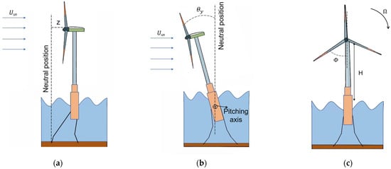
Figure 1. Schematic diagram of a spar-type floating horizontal-axial wind turbine (HAWT) with (a) surge motion, (b) pitch motion, and (c) front view.
Based on the rigid assumption of the wind turbine, the relative velocities of a blade element with a distance of 𝑟 from the rotational center of the blades can be calculated as follows [38][23]:
In Equations (8) and (9), 𝑈∞ is the inflow velocity perpendicular to the rotation plane of the HAWT and 𝜃𝑦 and 𝑧˙ show the pitch and heave responses of the floating HAWT. While 𝐻 is the height of the rotational center and 𝑟 is the radial distance of the blade section from the rotational center, 𝜙 presents the azimuth angle of a certain blade. 𝑎 and 𝑎’, on the other hand, are the axial and tangential induction factors, which are calculated in Equations (16) and (17). It is noted that the aerodynamic loads acting on the blade rely primarily on the relative velocity component perpendicular to the blade (𝑢) and in the vertical direction (𝑤), and hence the component along the blade (𝑣) is neglected. The inflow angle, which is key to calculating the angle of attack (AOA) and then for the induction factors, is therefore determined as follows:
The aerodynamic loads acting on the blades, specifically the lift and drag forces, are mainly determined by the AOA, the Mach number, and the Reynolds number. While the Mach number is typically small enough in the case of HAWT (usually less than 0.3) to be ignored, the Reynolds number interacts with the airfoil design of the blade to impact the aerodynamic load calculation. Nonetheless, it is commonly acknowledged that the AOA (𝛼𝑎𝑡𝑡𝑎𝑐𝑘), is the most influential factor in the estimation of the drag and lift forces acting on the blade [39,40][24][25], defined as the difference between the inflow angle and the 𝜃 (sum of the pitch angle (𝛽) and the twisting angle (𝜗) of the specific section), as follows:
With the known AOA, the drag (𝐶𝑑) and lift (𝐶𝑙) coefficients can be derived from a table containing the data accumulated from the experiment or full-set numerical simulation results [41][26]. In fact, it is found from the literature that Reynolds numbers [42][27], the general geometry of the blade [43][28], the use of end-plates [44][29], and other factors all influence the aerodynamic characteristics of the blade. Hence, it is necessary to obtain the drag and lift coefficient database specifically for the blade design under investigation. Given the inflow angle of 𝜑, the normal (𝐶𝑛) and tangential (𝐶𝑡) load coefficients are calculated as follows:
In addition, the thrust and torque acting on the rotating centre induced by a single blade are calculated as follows:
In Equations (14) and (15), 𝐹 is the thrust, 𝑀 is the torque, 𝑐(𝑟) shows the chord length as a function of the radial distance (𝑟), and 𝑅ℎ and 𝑅𝑏 are the radius of the hub and the radial distance of the blade tip, respectively. The axial and tangential induction factors are functions of the relative velocity, solidity, normal, and tangential load coefficients, as follows:
In Equations (16) and (17), 𝜎 is the solidity of the blade section and is defined as the ratio of the swept area and the corresponding control volume.
It is understandable that the aerodynamic loads estimated according to classic BEM theory are inaccurate in a number of aspects [45][30]. Consequently, there are several corrections reported in the literature to reduce the bias of the assumptions employed in the classic BEM theory (relevant details are available in [46][31]). For example, the Prandtl correction factor has been suggested to correct the unrealistic infinite blade section assumption [47][32], and the Glauert correction is suggested for cases where the axial induction factor is beyond 0.4 [6,34][18][19].
The calculation of the aerodynamic loads acting on the HAWT according to the BEM theory is in fact an iterative process starting with an assuming axial and tangential factor [48][33]. The AOA can then be calculated according to Equation (11), which leads to the estimates of lift and drag coefficients. Afterwards, the normal and tangential load coefficients are delivered to give the estimates of the induction factors in the current iteration, as shown in Equations (16) and (17). Such an iterative process continues until the residuals corresponding to both induction factors reduce below the specific thresholds. The ultimate estimates of the thrust and torque acting on the blades are then calculated according to Equations (14) and (15). Alongside this conventional approach, different algorithms have also been suggested, such as the simplification reported in [49][34].
References
- Vorpahl, F.; Schwarze, H.; Fischer, T.; Seidel, M.; Jonkman, J. Offshore Wind Turbine Environment, Loads, Simulation, and Design. WIREs Energy Environ. 2013, 2, 548–570.
- Lu, H.; Porté-Agel, F. Large-Eddy Simulation of a Very Large Wind Farm in a Stable Atmospheric Boundary Layer. Phys. Fluids 2011, 23, 065101.
- Churchfield, M.J.; Lee, S.; Michalakes, J.; Moriarty, P.J. A Numerical Study of the Effects of Atmospheric and Wake Turbulence on Wind Turbine Dynamics. J. Turbul. 2012, 13, N14.
- Pope, S.B. Turbulent Flows. Meas. Sci. Technol. 2001, 12, 2020–2021.
- Thordal, M.S.; Bennetsen, J.C.; Koss, H.H.H. Review for Practical Application of CFD for the Determination of Wind Load on High-Rise Buildings. J. Wind. Eng. Ind. Aerodyn. 2019, 186, 155–168.
- Mann, J. Wind Field Simulation. Probab. Eng. Mech. 1998, 13, 269–282.
- Mann, J. The Spatial Structure of Neutral Atmospheric Surface-Layer Turbulence. J. Fluid Mech. 1994, 273, 141–168.
- Hsieh, A.; Maniaci, D.C.; Herges, T.G.; Geraci, G.; Seidl, D.T.; Eldred, M.S.; Blaylock, M.L.; Houchens, B.C. Multilevel Uncertainty Quantification Using CFD and Openfast Simulations of the Swift Facility. In Proceedings of the AIAA Scitech 2020 Forum, Orlando, FL, USA, 6–10 January 2020; p. 1949.
- Hübner, G.; Pinheiro, H.; de Souza, C.; Franchi, C.; Da Rosa, L.; Dias, J. Detection of Mass Imbalance in the Rotor of Wind Turbines Using Support Vector Machine. Renew. Energy 2021, 170, 49–59.
- Somoano, M.; Battistella, T.; Rodríguez-Luis, A.; Fernández-Ruano, S.; Guanche, R. Influence of Turbulence Models on the Dynamic Response of a Semi-Submersible Floating Offshore Wind Platform. Ocean Eng. 2021, 237, 109629.
- Malik, H.; Almutairi, A. Modified Fuzzy-Q-Learning (MFQL)-Based Mechanical Fault Diagnosis for Direct-Drive Wind Turbines Using Electrical Signals. IEEE Access 2021, 9, 52569–52579.
- Pettas, V.; Costa García, F.; Kretschmer, M.; Rinker, J.M.; Clifton, A.; Cheng, P.W. A Numerical Framework for Constraining Synthetic Wind Fields with Lidar Measurements for Improved Load Simulations. In Proceedings of the AIAA Scitech 2020 Forum, Orlando, FL, USA, 6–10 January 2020; p. 0993.
- Pokhrel, J.; Seo, J. Statistical Model for Fragility Estimates of Offshore Wind Turbines Subjected to Aero-Hydro Dynamic Loads. Renew. Energy 2021, 163, 1495–1507.
- Jonkman, B.J. TurbSim User’s Guide: Version 1.50. Available online: https://www.osti.gov/biblio/965520 (accessed on 3 September 2023).
- Zhou, Y.; Xiao, Q.; Liu, Y.; Incecik, A.; Peyrard, C.; Wan, D.; Pan, G.; Li, S. Exploring Inflow Wind Condition on Floating Offshore Wind Turbine Aerodynamic Characterisation and Platform Motion Prediction Using Blade Resolved CFD Simulation. Renew. Energy 2022, 182, 1060–1079.
- Salzmann, D.C.; Van der Tempel, J. Aerodynamic Damping in the Design of Support Structures for Offshore Wind Turbines. In Proceedings of the Paper of the Copenhagen Offshore Conference, Copenhagen, Denmark, 23–25 November 2021.
- Moriarty, P.J.; Hansen, A.C. AeroDyn Theory Manual. Available online: https://www.osti.gov/biblio/15014831 (accessed on 9 September 2023).
- Bai, C.J.; Wang, W.C. Review of Computational and Experimental Approaches to Analysis of Aerodynamic Performance in Horizontal-Axis Wind Turbines (HAWTs). Renew. Sustain. Energy Rev. 2016, 63, 506–519.
- Subbulakshmi, A.; Verma, M.; Keerthana, M.; Sasmal, S.; Harikrishna, P.; Kapuria, S. Recent Advances in Experimental and Numerical Methods for Dynamic Analysis of Floating Offshore Wind Turbines—An Integrated Review. Renew. Sustain. Energy Rev. 2022, 164, 112525.
- Sun, X.; Zhou, D. Review of Numerical and Experimental Studies on Flow Characteristics around a Straight-Bladed Vertical Axis Wind Turbine and Its Performance Enhancement Strategies. Arch. Comput. Methods Eng. 2022, 29, 1839–1874.
- Sant, T.; Cuschieri, K. Comparing Three Aerodynamic Models for Predicting the Thrust and Power Characteristics of a Yawed Floating Wind Turbine Rotor. J. Sol. Energy Eng. 2016, 138, 031004.
- Wu, C.H.K.; Nguyen, V.T. Aerodynamic Simulations of Offshore Floating Wind Turbine in Platform-Induced Pitching Motion. Wind Energy 2017, 20, 835–858.
- Micallef, D.; Rezaeiha, A. Floating Offshore Wind Turbine Aerodynamics: Trends and Future Challenges. Renew. Sustain. Energy Rev. 2021, 152, 111696.
- Lee, H.; Lee, D.-J. Effects of Platform Motions on Aerodynamic Performance and Unsteady Wake Evolution of a Floating Offshore Wind Turbine. Renew. Energy 2019, 143, 9–23.
- Wen, B.; Tian, X.; Dong, X.; Peng, Z.; Zhang, W. Influences of Surge Motion on the Power and Thrust Characteristics of an Offshore Floating Wind Turbine. Energy 2017, 141, 2054–2068.
- Oukassou, K.; El Mouhsine, S.; El Hajjaji, A.; Kharbouch, B. Comparison of the Power, Lift and Drag Coefficients of Wind Turbine Blade from Aerodynamics Characteristics of Naca0012 and Naca2412. Procedia Manuf. 2019, 32, 983–990.
- Almukhtar, A.H. Effect of drag on the Performance for an Efficient Wind Turbine Blade Design. Energy Procedia 2012, 18, 404–415.
- Liu, Y.-C.; Hsiao, F.-B. Aerodynamic Investigations of Low-Aspect-Ratio Thin Plate Wings at Low Reynolds Numbers. J. Mech. 2012, 28, 77–89.
- Villeneuve, T.; Boudreau, M.; Dumas, G. Lift Enhancement and Drag Reduction of Lifting Blades through the Use of End-Plates and Detached End-Plates. J. Wind Eng. Ind. Aerodyn. 2019, 184, 391–404.
- Jeon, M.; Lee, S.; Lee, S. Unsteady Aerodynamics of Offshore Floating Wind Turbines in Platform Pitching Motion Using Vortex Lattice Method. Renew. Energy 2014, 65, 207–212.
- Hansen, M.O. Aerodynamics of Wind Turbines: Rotors, Loads and Structure; Earthscan: Oxford, UK, 2000; Volume 17.
- Shen, W.Z.; Mikkelsen, R.; Sørensen, J.N.; Bak, C. Tip Loss Corrections for Wind Turbine Computations. Wind Energy 2005, 8, 457–475.
- Hansen, M. Aerodynamics of Wind Turbines; Routledge: Oxford, UK, 2015.
- Ning, S.A. A Simple Solution Method for the Blade Element Momentum Equations with Guaranteed Convergence. Wind Energy 2014, 17, 1327–1345.
More