The F-channel platform will contribute to enhancing the active management of the power system for TSO–DSO coordination by using AI methods and cloud calculation engines. However, in order to accomplish this, certain requirements had to be satisfied, the first of which was the availability of comprehensive models of climate data. The convenience of having these models at hand made it possible to forecast the different parameters that are important from the perspective of the SOs. For example, the ability to modify the AI algorithms was made possible by the reasonably high-resolution predictions of wind speeds and insolation patterns ^[1][2][3][4][36,37,38,39] and connecting those predictions with the behavior of the generation units in the power system in a way that has never been seen before. In addition, the power demand estimates as well as the possibility of conductor icing and storms that could compromise the system’s operational reliability are important. These can be viewed as the concepts guiding the improvements and innovations made to the flexibility channel ^[5][6][7][40,41,42].

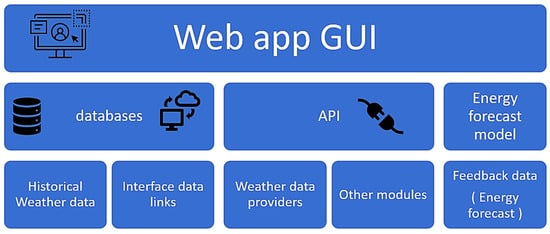
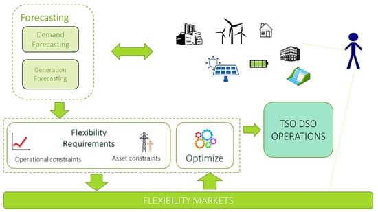
To enable the flawless execution of the foreseen processes and calculations, while maintaining the desired level of the user-friendliness, it was necessary to find the optimal engines for performing the analyses that can be paired with the appropriate UI. To make that happen, the cloud-computing engines were selected for the role. The diagram provided in Figure 1 provides an overview of the basic architecture of the proposed web application, while Figure 12 presents the expected role of this platform in the flexibility market.

The TSO and DSO in Greece will share flexibility resources and coordinate their efforts to meet their augmenting regional challenges through grid services stemming from prosumers, aggregators, suppliers, and producers, while at the same time optimizing the use of network assets and big-data-processing tools for network predictability and observability. F-channel modules will incorporate “prosumers”, “aggregators”, and their forms of participation in the energy mix and flexibility provision, such as flexibility providers/storage owners/EV charging station operators. Forecasting engines can be used to include consumers by using aggregations based on the geographic location of POIs. The production capability of local consumers can be precisely included in the forecasting system. Modeling the RES capacities of local industries and families allows for the planning of consumer activities. Customers can participate by entering their daily, weekly, or hourly needs. This strategy can be particularly helpful for local companies that have time-sensitive, repetitive processes with known steady loads. They can benefit from demo with knowledge if (and when) they can use local capacity. Furthermore, by tracking their needs, demo can propose installing RES capacity if none is present for the consumer.

As suggested by Figure 1 and Figure 12, the F-channel platform was designed to pay great attention to finding the best possible combination of the technical proficiency of the functionalities and easy-to-adapt-to UI, affording the users the best possible experience. At the same time, it will satisfy the standards set by the modern tools that are applied for the system analyses by the interested parties. Regarding the storage of the data needed for conducting the foreseen procedures, databases and storage accounts were required. The allocated computing resources have been divided into two groups: continuously allocated ones and ones allocated per computation.

Furthermore, it was also necessary to specify the way in which the required databases would be structured, and for this purpose, it was decided to use the traditional RDBM rational model. The geospatial data display was provided by the middleware software architecture supporting WMS and WFS. The server infrastructure security was paid special attention because, in recent years, there have been an increasing number of data leaks and hacker attacks, even on some of the biggest and most well-defended companies whose expertise is in power systems and their management. As a result, the security of the server infrastructure has become more and more important. Thus, the server access codes required encryption using relevant SSH keys. Additionally, access to the various sections of the platform was limited, such that users could only access the designated IP address ranges. Following that strategy, user-side web application access had to be restricted to verified user accounts, and each user could only view the relevant page on the F-channel platform, based on the specified type provided to them.

For the purpose of enabling the foreseen functionalities of the F-channel platform in the best possible way, it was also necessary to obtain the appropriate amount of input data from the Greek system operators, both in the form of the exact values related to the specifications of the system in the regions of interest for the projects and in the form of experience regarding the practical manner in which certain processes that are supposed to be included in the platform take place. In ^[8][9][34,35], the following data requests have been stated:

• network models’ data
• geospatial data
• technical data for wind turbines
• technical data for solar parks
• technical data for selected overhead lines.

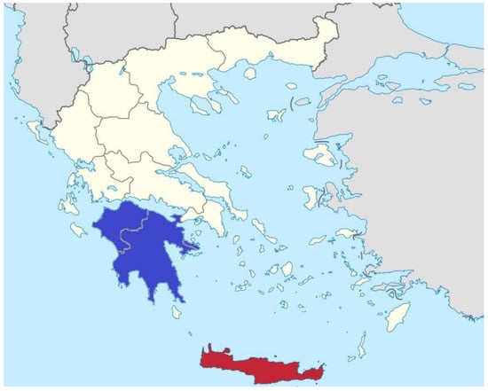
The data had to be delivered for the area of interest of Greece, which included the geographic regions of Crete Island and the Peloponnese Peninsula. The geographic map of this region (with Peloponnese in blue and Crete in red) can be seen in Figure 23.

Due to the interconnection between Crete and Peloponnese, the network that was taken into consideration for the chosen region includes the grid at all voltages, from 400 kV down to 20 kV, for a total of 50 substations in Peloponnese and 1 substation in Crete. Out of the 50 substations in the Peloponnese, 28 had a connected load and 22 had a connection with renewable energy sources. Virtual customers served as the demo’s clients. The following numbers are accurate when it comes to the resources considered in the current work:

• 161 overhead lines (OHL)
• 13 solar power plants (SPPs) (additional SPPs were originally planned, but the necessary data were only available for 13 SPPs)
• 37 wind power plants (WPPs).

The hourly production power values for all of the mentioned WPPs and SPPs were gathered over a five-year period and used. These values cannot be demonstrated in the current work due to problems with data confidentiality. In addition, data were gathered at the EU level for instances of critical wind-icing and precipitation combinations as well as wind–precipitation combinations, validating the platform’s utility for forecasting of critical weather circumstances that could result in severe system states. Even if that were not the case, one could still find the routes of the system’s lines on the map services available online. The routes of the lines in the system have typically been provided by the system operators.

The goal of the work presented here is how the F-channel platform can manage outages and ensure the power system’s resilience during extreme weather conditions. The extreme weather conditions fulfill some specific criteria that can affect the power system. The weather parameters that can cause critical system situations are:

• high wind speeds (over 12 m/s)
• low barometric pressure (under 960 mbar)
• cloud cover
• lightning
• icing of the power lines
• low wind speeds (under 5 m/s) combined with the appearance of clouds (simultaneous halting of the production of wind and solar units).

If operators spot that critical system situations can occur due to the extreme conditions (fulfilling some of the above-mentioned weather parameters), then the course of action needs to be chosen. Such a scenario is presented in Section 4 of this paper.

Before any kind of activity was performed in the creation of the “F-channel” platform, it was necessary to determine the best tool that could be used for managing the databases containing the information needed for the successful operation of the platform. For this role, MySQL 8.0 was selected. The selection was based on the fact that the work in this database is quite intuitive, and a majority of experts are somewhat familiar with it already due to its wide range of applications and adaptability, as well as its nature as an open-source tool. This means that it is possible for anyone to use this software and modify it according to their own preferences and the task for which they intend to use it. Moreover, it is well-known for data security (with the possible leaks and the cyber-security issues posing more and more of a threat in the era of digitalization) and efficiency, ensuring the smooth running of the processes for which the MySQL database is applied.

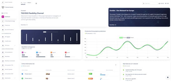
In the F-Channel GUI platform, there are five types of users (accounts): FSP/aggregator, DSO, TSO, market operator, and guest. The most important section of this platform and, probably, the section on which the user will spend the majority of their time, would be the dashboard. The dashboard can be seen as a sort of homepage that is first opened as soon as the log-in process is successfully completed. What is included in it, however, varies depending on the role that is taken by the user, with the “need-to-know” principle applied when designing the dashboards for each of the five specified types. The sole exception from this rule is the pages for the TSO and for the DSO, which are quite similar, with the main difference between them being the set of products relevant for the respective system operators. This exact window is shown in Figure 34, where the functionalities offered to the system operators can be seen.

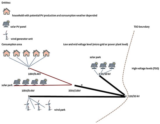
When choosing which parts of the system, such as individual homes or single production units in the power plants, need to be modeled to the lowest-level entities, special consideration must be given. An understanding of the necessary modeling proficiency for each and every energy market participant can be gained from Figure 45.

The goal of the modeling process was to enable the F-channel platform’s users—primarily the SOs—to obtain information about the current system state that was, until now, inaccessible to them, i.e., real-time alterations in each household’s behavior, as shown in Figure 45. The operators have all the potentially relevant information needed to make informed decisions and come to successful conclusions by providing them realistic data on the system entities that interest them. As a result, the decisions made would be in keeping with the needs of everyone involved in the system as a whole. After all applications were gathered, carefully examined, and assessed, the GEOGRID (GEOreferenced GRID simulation model) solution was chosen, and it is extensively detailed in the following section.

The main targets of the GEOGRID solution were the development of the power system simulation model, including the voltage levels down to the lowest ones, and the creation of the GIS server, which would then be used for the visualization of the obtained results. In addition, another goal that was defined was the development of an appropriate GUI that would both hold the option of introducing all the achievements of this solution to the users and fit into the overall environment of the F-channel platform, especially considering the desired levels of simplicity, intuitiveness, and efficiency.

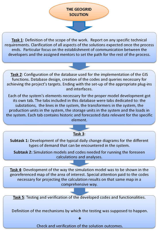
The activities that had been foreseen for GEOGRID were, after defining the main targets, divided into five main tasks. A short description of each of those five tasks can be found below, where it needs to be underlined that, even though the tasks were mostly performed in sequential order, there were some occasions in which the work on several tasks took place simultaneously for the purposes of optimal usage of the resources that were at the disposal of the solution developers. The tasks expected from the GEOGRID are depicted in the flow chart of Figure 56.

In the scope of the GEOGRID solution, it was, before conducting any other activities, necessary to determine the load profiles that can be assigned to the specific types of demand in the system. This was necessary to determine related to the number of consumption categories that would be considered, so that the number was high enough to successfully cover all of the major types of loads that exist in the system, but low enough to justify the introduction of the load categories at all. Hence, it was determined that it is optimal for the demand to be divided into four specific types:

• household demand
• industry demand
• commercial services demand
• electric vehicles demand.

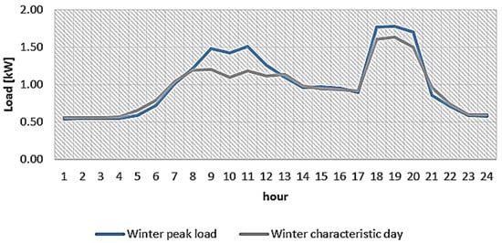
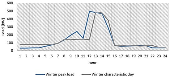
For each of these demand types, it was then necessary to figure out the daily diagram, by which the power of that type of load would vary throughout the day. To make that happen, the data obtained from the measurements were combined with the statements and estimations provided in the literature dealing with similar topics. In line with the order in which the different types of load were mentioned in the list above, the first kind of consumption that was analyzed in detail by the GEOGRID solution developers was the household demand, typical for rural areas in which the industry is not developed yet, as well as for the urban areas that are not foreseen as the ones in which large factories will be located, i.e., areas that will not be a part of the city’s industrial zone in the future. The typical daily diagram of this type of demand can be seen in Figure 67, reflecting the behavior of household consumption on a characteristic day of winter, but also on the day of the measured winter peak of the demand power. These are marked with different colors in Figure 67, with the blue color corresponding to the demand’s behavior on the day of the winter peak regime and the grey line marking the change in the demand’s power during the approximate winter characteristic day.

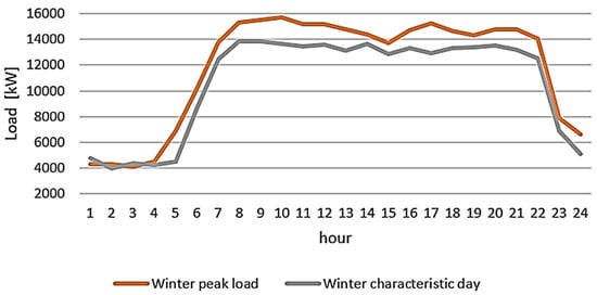
The next type of demand that was considered in the scope of the third task of the GEOGRID solution was industry consumption, typical for a major industrial zone in which a large number of factories is located. This can either be the zones in the rural areas, located there to preserve the ecological standards of the air and water quality in the nearby towns, or they can be placed near the outskirts of the cities, depending on the types of processes that take place in the facilities in the industrial zone and the decisions and priorities of the local governments. For this demand’s behavior to be properly illustrated, Figure 78 is presented, with the different colors of the lines once again corresponding to the chosen days of the winter period. The orange and gray lines, respectively, show the valid data for the winter peak load day and the winter characteristic day.

The third type of demand that will be briefly explained here is the commercial load, for which the daily diagram of power variation can be seen in Figure 89. This category of demand corresponds, among other consumers that cannot be placed in the last two types, to the administration offices, which is the very example upon which the figure provided below was based.

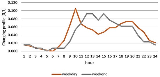
The fourth and final type of consumer demand that was considered separately in the scope of this work was the demand related to the charging process of electric vehicles. For this demand type, it needs to be stated that it was not present in the literature until recently, but with the number of electric vehicles on the streets increasing daily, it became a necessity to separate it from the other three categories. Along with the different types of variation throughout the day, what also makes this category of demand so different from the other three is the fact that its power does not depend so much on the weather conditions or the season of the year, for instance (both of these are rather prominent factors for household demand), but on whether the observed day belongs to the weekend or not. This is understandable, as the load related to this demand type and its distribution during the day change with the number of people going to work or on fieldtrips. In line with this conclusion, the diagram in Figure 910 contains two lines, but this time, the orange color marks the weekday’s load behavior, and the grey color symbolizes the behavior of the load during the weekend, which is different from the concept used for the previous three figures.

Along with these diagrams and the comments regarding the practical situations in which all these demand types can be encountered, the GEOGRID also contains a discussion regarding the flexibility potential that every demand type can offer to the system, based on the daily diagrams referring to each of these types. Here, it can be seen that the peaks of this demand are in the morning and in the evening, when people are going to work and returning from work, respectively. For the morning peak, the vehicles are commonly charged in the buildings in which the drivers of these vehicles work, so the smart charger system could be implemented to distribute the load throughout the working hours. On the other hand, during the evening peak, during which vehicles are typically charged in the homes of the drivers, the appropriate tariff system could help spread the load throughout the night.

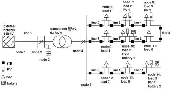
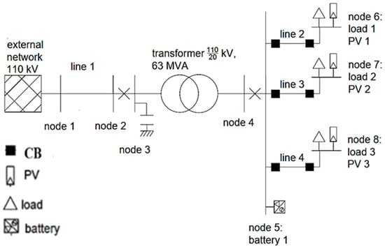
With the demand profiles out of the way, the developers of the GEOGRID solution moved to the next level, encompassing the development of the simulation models of the various microgrids that were later combined with the model of the Crete transmission system based on the data delivered by IPTO, so the model of the entire area of interest could be established. The approach that was adopted in this step was that each of the microgrids that were modeled needed to correspond to one of the load profiles developed in the previous part of this task. Therefore, four different microgrid models have been created, with Figure 101 providing insight into the grid corresponding to household demand, the first out of the mentioned four types.

This example of the microgrid includes all the entities that can be encountered in the common segment of the distribution system that contains the household load, with the 110 kV transmission system here in the form of the appropriate equivalent network. The provided diagram shows that, along with this equivalent, the microgrid contains the transformer connecting the transmission and distribution grids, the bus in the 20 kV part of the 110/20 kV substation, and the branches that go from that busbar toward the loads in the observed section of the system. For this instance, it was decided that the load in the selected microgrid can be supplied by three feeders, with each of them containing three nodes with the demand attached. Two of the feeders are connected by an additional line (line 5 in Figure 110), but the switch on that line is treated as turned off in the normal operation, matching the typical approach used when planning the distribution grid. Along with the nine loads, the created microgrid also contains four PV units (attached to nodes 7, 8, 10, and 14), as well as two batteries (attached to nodes 10 and 14). Of course, the microgrids that were developed to correspond to the remaining three types of demand kept some of the elements presented here the same, such as the external grid, while bringing enough variation to show different schematics of the distribution system’s operation. This will be shown in the following lines, each dealing with one of the microgrid types developed for the solution.

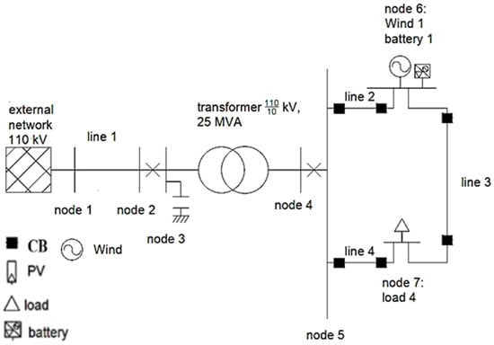
In the same manner, Figure 112 shows the schematic of the microgrid that has been created for industry consumption. As can be seen, the concept of energy provision for the needs of households is rather different than the one used for the supply of energy for large industrial consumers, with the most obvious difference being the fact that, in the case of household consumption, there is more than one consumer that is supplied via a HV/MV transformer. However, the demand that belongs to some of the larger industrial facilities is often supplied via its own transformer, as illustrated in Figure 112. Alongside the difference regarding the transformer, the microgrid that was created for showcasing the situation related to the industry also contains a single node with a load (shown in the bottom part of the schematic) and another node, to which the system, composed of the wind generation unit and the battery, is connected (shown in the upper part of the schematic). This concept of the microgrid reflects the modern-day tendency of large industrial facilities to have at least some sort of energy production in the close vicinity of the load, with the storage system added for at least partial damping of the production power variations of the wind generation unit. What should also be underlined is the fact that each of the two mentioned nodes is radially connected to the 10 kV node in the 110/10 kV substation, but that there is also an additional link that connects those two nodes directly, numbered 3 in Figure 112. This link is switched off in normal operation, following the same logic as the one described for the household load, and serves as a voucher of the uninterrupted supply in case of an outage of one of the other 10 kV lines. For the industrial load, this can be even more important than for households, due to the chemicals typically used in the industry today.

Figure 123 provides a schematic of the microgrid exclusively used for commercial consumption. Once again, a comparison can be made between the microgrid created for the sake of including the load of the commercial service providers and the grids made for illustrating the behavior of the loads for the previous two cases and, once again, some differences can be spotted. The first of these is the fact that, in this case, each of the different loads of the commercial service providers has its own feeder, connecting it to the 20 kV bus in the 110/20 kV substation. However, this time, there is no additional line that could serve as a backup in case one of the lines gets tripped, so the uninterrupted supply of energy is not guaranteed. This can be tolerated here since the load itself is less sensitive than, for example, industrial facilities, where even the shortest pause in the supply could cause a disaster and put not only the facility but also the surrounding area at risk of a natural catastrophe. It is presumed that each of the three commercial loads is equipped with its own solar unit and that the energy storage (assumed to be the battery) is common for all of them and located at the 20 kV bus in the 110/20 kV substation. The external 110 kV grid is, in line with what was already said, present here as well.

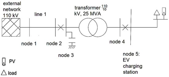
Finally, Figure 134 shows the schematic of the microgrid for the EV charging demand. Even though this schematic appears to be the simplest of the four, it becomes a bit more complicated than that if the load that is attached to node 5 of this diagram does not represent a single charging socket but all the sockets that are in the same facility are taken into consideration. In addition to this, it was assumed that this charging station is equipped with a solar production unit, ensuring maximal potential for the provision of flexibility to the system by applying the combination of the generation in the solar unit and the load of the EV chargers.

Now, with the descriptions of each of the four microgrids created for the purposes of the GEOGRID solution out of the way, a couple of points regarding the usage of these microgrids in the models and calculations must be made. First, the apparent discrepancy between the voltage levels used in the models of microgrids shown here and the real-life situation in Crete needs to be addressed. Namely, the models from the solution use the 110 kV level as the HV side of the transformers, whereas the voltage of the transmission grid in Crete is 150 kV, so some readers could wonder if these models could even be integrated with the rest of the Crete grid. To clarify this, one must start with the fact that each of the microgrid models has only two elements for which the HV level is relevant: the external grid element and the HV/MV transformer. By simply changing the parameters of this transformer, it could easily be modified to be suitable for connecting the HV side to the 150 kV level. On the other hand, an external grid is nothing more than a fictitious element that would, in case the model of the microgrid merged with some other model, most likely end up being deleted.

That was the exact case with the situation in which the unified model of the Crete grid needed to be created. To make that happen, the authors of the GEOGRID solution took the accurate model of the 150 kV transmission grid in the region of interest and then, instead of combining it with the accurate model of the distribution grid, used the developed microgrids (modified to be able to be connected to the 150 kV level) as the proxies of the distribution system. This step had to be completed in that way due to the unavailability of high-quality input data related to the distribution system at the time of the creation of the unified model. Of course, if the input data regarding the distribution grid were available, it would be better to use those instead of simulating it with the microgrids shown here. However, the mentioned situation at the time of the unified model’s creation left the authors with no other option besides using the microgrids. This was achieved by taking each of the 150 kV nodes to which part of the distribution system should be connected and attaching one of the microgrids to it instead. The unified model, created in the described way, will be shown in the later part of this section. Before that, the codes that were written to add the necessary features to the solution must be briefly explained.

The information provided in the sheets varied depending on the type of element to which that sheet was dedicated; thus, for example, the sheet related to the external grid contained solely the power flow from the external grid to the microgrid. The sheets related to the lines and the transformers, on the other hand, contained the flows over those elements, measured on both the starting and ending buses. The sheet dedicated to the buses finally contained the columns for the active and reactive power demand in every bus, as well as the value of the voltage in those nodes and the phase angles of those voltages.

With this, the entirety of the activities foreseen for the first three tasks of the GEOGRID have been completed, allowing the developers to move on to the last two tasks related to this process. Furthermore, what needed to be completed was the creation of the simulation model that would cover the entire island of Crete (the 150 kV grid, the transformers connecting that grid, the distribution voltage levels, the distribution level microgrids, and the generation capacities and demand). In accordance with that, this task was divided into four sub-tasks before starting the actions upon its completion:

• creation of the unified model of the selected part of the system on Crete Island
• modification of the codes for the load flow calculation to run the analysis on the unified model
• projection of the created unified model on the appropriate map
• enabling the presentation of the obtained results on the map in a comprehensive manner.

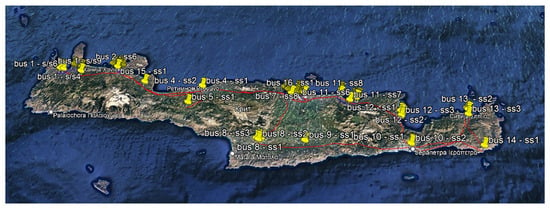
The first two sub-tasks here can be seen as the upscaling of the achievements already included in the third task of GEOGRID. Therefore, attention will be given to the latter two sub-tasks, with the georeferenced map of the entire grid of Crete Island (all voltage levels) shown in Figure 145.

Here, it can also be seen that, once the map was zoomed in to the scale enough, the yellow pins showed the locations of the distribution level facilities as well, and the blue lines, marking the routes of the distribution power lines, also became visible. However, to make the application of this functionality even more user-friendly, an additional option was added, allowing the potential users to select the layers that the map will include, with one of the layers containing, for example, the 150 kV grid in the area of interest. By switching that layer off, the user can put more emphasis on the state of the distribution grid in case the report on which they are currently working requests it. With this sub-task completed, the sole thing remaining to be completed before the official finalization of Task 4 was the development of the way the results of load flow calculations could be included in the grid map. This was one of the most demanding challenges put before the authors of the GEOGRID solution, but also one of the main advancements that aided GEOGRID in being selected during the Open Call process. Namely, the proper resolution of this issue also meant that the results of the performed analyses could be shown in a manner understandable both to the engineers that work in the software tools for these calculations daily and to the public, where the presentations of the most prominent conclusions of these analyses could be held. This improvement was seen as one of the main assets that could enhance communication between the power industry and the authorities, explaining why this sub-task was set as one of the highest priorities by the mentors assigned to the project’s developers.

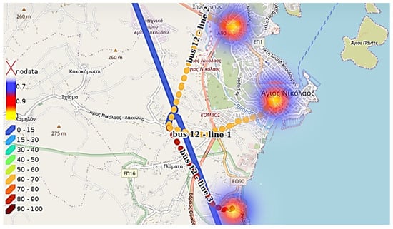
For this to be accomplished, the developers first needed to choose the way in which the power flows and the voltages in the selected part of the georeferenced map would be presented, with the option of having the color schemes for both of those parameters’ surfaces as the best ones in the end. Therefore, for the lines, the different colors of their representation refer to the various loadings, with the blue shades showing the relatively low loading of the lines and the red shades indicating the high loading of the lines. For the nodes and their voltages, a similar logic was used: if the color surrounding the node was in the blue part of the spectrum, the voltage of that node was on the low side, and if the color was closer to the yellow shades, that meant that the voltage of the node was closer to the rated value. This approach may seem confusing when described in this way, but it is rather intuitive and simple to understand, which can be confirmed in Figure 156, showing the loadings of the lines and voltages in the distribution grid around Agios Nikolaos. Line 3 from bus 12 is more loaded than lines 1 and 2 from the same node. This can easily be seen in Figure 156, since that line is colored in red, whereas the other two are marked in yellow.

Finally, the tests and verifications (Task 2 of Figure 56), necessary before the activities regarding the development of the GEOGRID solution were considered finished, took place in the form of checking the four predefined criteria:

• confirmation of the accuracy of the used input data
• confirmation of the precision of the conducted calculations
• confirmation of the replicability of the obtained results
• confirmation of the reliability of the graphical representation.