The application of various machine learning techniques for predicting customer churn in the telecommunications sector is explored. Researchers utilized a publicly accessible dataset and implemented several models, including Artificial Neural Networks, Decision Trees, Support Vector Machines, Random Forests, Logistic Regression, and gradient boosting techniques (XGBoost, LightGBM, and CatBoost). To mitigate the challenges posed by imbalanced datasets, researchers adopted different data sampling strategies, namely SMOTE, SMOTE combined with Tomek Links, and SMOTE combined with Edited Nearest Neighbors. Moreover, hyperparameter tuning was employed to enhance model performance. Resarchers' evaluation employed standard metrics, such as Precision, Recall, F1-score, and the Receiver Operating Characteristic Area Under Curve (ROC AUC). In terms of the F1-score metric, CatBoost demonstrates superior performance compared to other machine learning models, achieving an outstanding 93% following the application of Optuna hyperparameter optimization. In the context of the ROC AUC metric, both XGBoost and CatBoost exhibit exceptional performance, recording remarkable scores of 91%. This achievement for XGBoost is attained after implementing a combination of SMOTE with Tomek Links, while CatBoost reaches this level of performance after the application of Optuna hyperparameter optimization.
- machine learning
- churn prediction
- SMOTE
- imbalanced data
- hyperparameter optimization
- Optuna
- Boosting techniques
- Bagging techniques
- classification methods
- ensemble techniques
1. Introduction
-
Providing a comprehensive definition of binary classification machine learning techniques tailored for imbalanced data.
-
Conducting an extensive review of diverse sampling techniques designed to address imbalanced data.
-
Offering a detailed account of the training and validation procedures within imbalanced domains.
-
Explaining the key evaluation metrics that are well-suited for imbalanced data scenarios.
-
Employing various machine learning models and conducting a thorough assessment, comparing their performance using commonly employed metrics across three distinct phases: after applying feature selection, after applying SMOTE, after applying SMOTE combined with Tomek Links, after applying SMOTE combined with ENN, and after applying Optuna hyperparameter tuning.
| Acronym | Meaning |
|---|---|
| ANN | Artificial Neural Network |
| AUC | Area Under the Curve |
| BPN | Back-Propagation Network |
| CatBoost | Categorical Boosting |
| CNN | Condensed Nearest Neighbor |
| DT | Decision Tree |
| ENN | Edited Nearest Neighbor |
| LightGBM | Light Gradient Boosting Machine |
| LR | Logistic Regression |
| ML | Machine Learning |
| RF | Random Forest |
| ROC | Receiver Operating Characteristic |
| SMOTE | Synthetic Minority Over-Sampling Technique |
| SVM | Support Vector Machine |
| XGBoost | eXtreme Gradient Boosting |
2. Machine Learning Techniques for Customer Churn Prediction
2.1. Artificial Neural Network
2.2. Support Vector Machine
2.3. Decision Tree
2.4. Logistic Regression
2.5. Ensemble Learning
2.5.1. Bagging

Random Forest

-
Sample nn training examples, Xb.YbbXb.Yb.
-
Train a classification tree (in the case of churn problems) fbfb b on the samples Xb.YbbXb.Yb.
2.5.2. Boosting

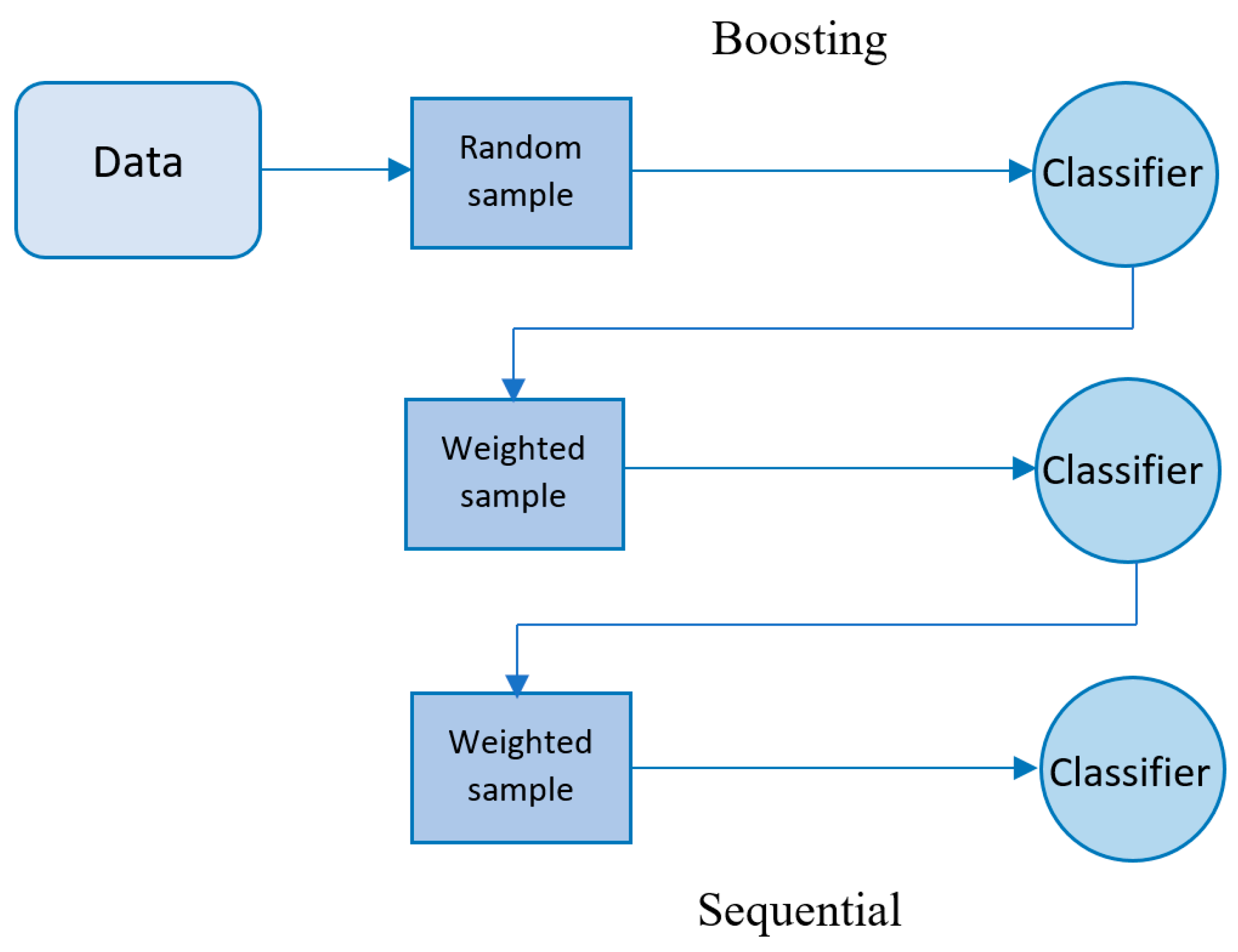
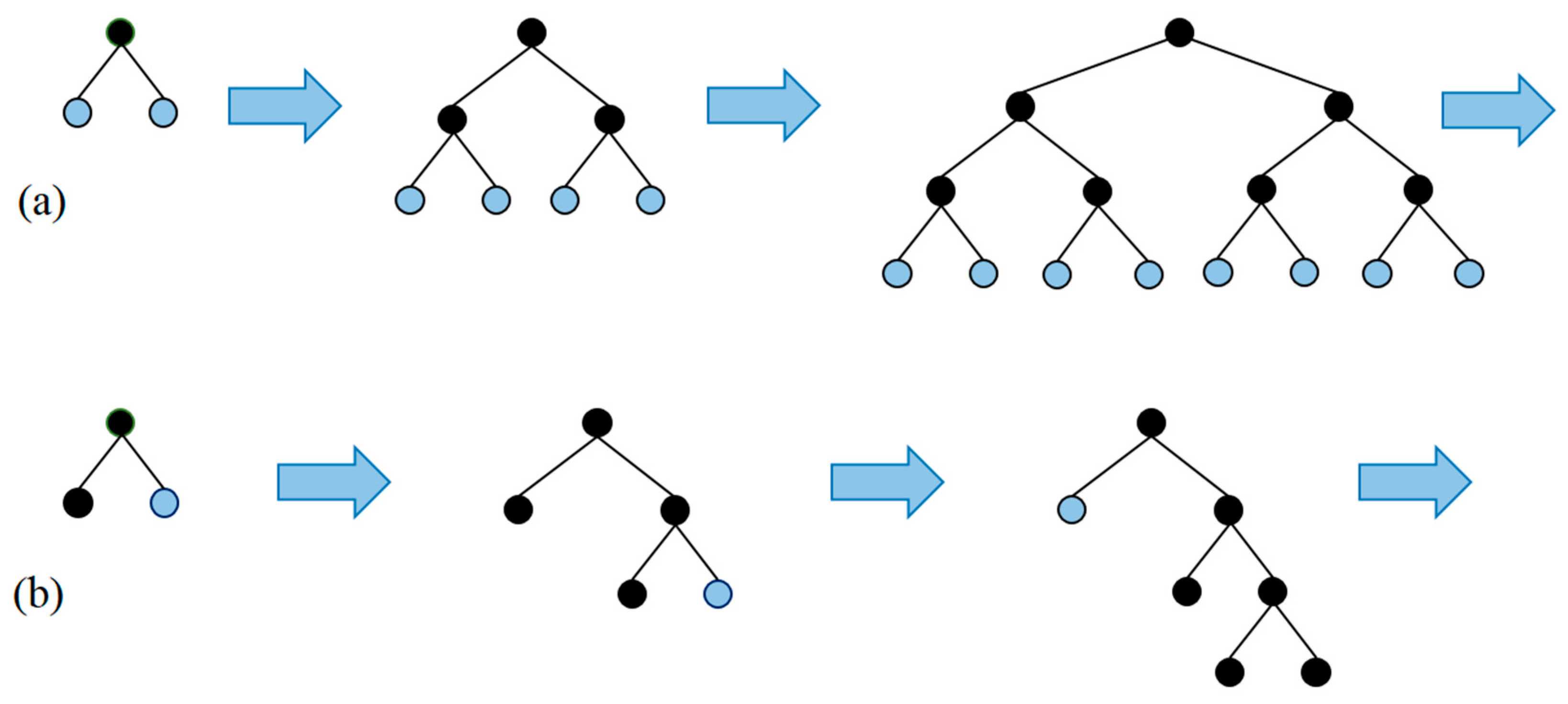
The Famous Trio: XGBoost, LightGBM, and CatBoost
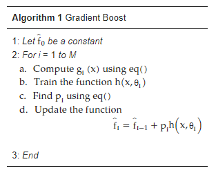
| Algorithm 1 Gradient Boost |
| 1: Let f̂ 0f^0 be a constant 2: For i = 1 to M a. Compute gi(x) using eq() a. Compute gix using eq() b. Train the function h(x,θi) b. Train the function h(x,�i) c. Find pi using eq() c. Find pi using eq() d. Update the function d. Update the function f̂ i=f̂ i−1+pih(x,θi)f^i=f^i−1+pih(x,�i) 3: End |


-
To randomly divide the records into subsets,
-
To convert the labels to integer numbers,
-
To transform the categorical features to numerical features, as follows:
References
- Cost of Customer Acquisition versus Customer Retention; The Chartered Institute of Marketing: Cookham, UK, 2010.
- Eichinger, F.; Nauck, D.D.; Klawonn, F. Sequence mining for customer behaviour predictions in telecommunications. In Proceedings of the Workshop on Practical Data Mining at ECML/PKDD, Berlin, Germany, 18–22 September 2006; pp. 3–10.
- Prasad, U.D.; Madhavi, S. Prediction of churn behaviour of bank customers using data mining tools. Indian J. Market. 2011, 42, 25–30.
- Keramati, A.; Ghaneei, H.; Mirmohammadi, S.M. Developing a prediction model for customer churn from electronic banking services using data mining. Financ. Innov. 2016, 2, 10.
- Scriney, M.; Dongyun, N.; Mark, R. Predicting customer churn for insurance data. In International Conference on Big Data Analytics and Knowledge Discovery; Springer: Cham, Switzerland, 2020.
- De Caigny, A.; Coussement, K.; De Bock, K.W. A new hybrid classification algorithm for customer churn prediction based on logistic regression and decision trees. Eur. J. Oper. Res. 2018, 269, 760–772.
- Kim, K.; Jun, C.-H.; Lee, J. Improved churn prediction in telecommunication industry by analyzing a large network. Expert Syst. Appl. 2014, 41, 6575–6584.
- Ahmad, A.K.; Jafar, A.; Aljoumaa, K. Customer churn prediction in telecom using machine learning in big data platform. J. Big Data 2019, 6, 28.
- Jadhav, R.J.; Pawar, U.T. Churn prediction in telecommunication using data mining technology. IJACSA Edit. 2011, 2, 17–19.
- Radosavljevik, D.; van der Putten, P.; Larsen, K.K. The impact of experimental setup in prepaid churn prediction for mobile telecommunications: What to predict, for whom and does the customer experience matter? Trans. Mach. Learn. Data Min. 2010, 3, 80–99.
- Richter, Y.; Yom-Tov, E.; Slonim, N. Predicting customer churn in mobile networks through analysis of social groups. In Proceedings of the 2010 SIAM International Conference on Data Mining, Columbus, OH, USA, 29 April–1 May 2010; Volume 2010, pp. 732–741.
- Amin, A.; Shah, B.; Khattak, A.M.; Moreira, F.J.L.; Ali, G.; Rocha, A.; Anwar, S. Cross-company customer churn prediction in telecommunication: A comparison of data transformation methods. Int. J. Inf. Manag. 2018, 46, 304–319.
- Tsiptsis, K.; Chorianopoulos, A. Data Mining Techniques in CRM: Inside Customer Segmentation; John Wiley & Sons: Hoboken, NJ, USA, 2011.
- Joudaki, M.; Imani, M.; Esmaeili, M.; Mahmoodi, M.; Mazhari, N. Presenting a New Approach for Predicting and Preventing Active/Deliberate Customer Churn in Tel-ecommunication Industry. In Proceedings of the International Conference on Security and Management (SAM), Las Vegas, NV, USA, 18–21 July 2011; The Steering Committee of the World Congress in Computer Science, Computer Engineering and Applied Computing (WorldComp): Athens, GA, USA, 2011.
- Amin, A.; Al-Obeidat, F.; Shah, B.; Adnan, A.; Loo, J.; Anwar, S. Customer churn prediction in telecommunication industry using data certainty. J. Bus. Res. 2019, 94, 290–301.
- Shaaban, E.; Helmy, Y.; Khedr, A.; Nasr, M. A proposed churn prediction model. J. Eng. Res. Appl. 2012, 2, 693–697.
- Khan, Y.; Shafiq, S.; Naeem, A.; Ahmed, S.; Safwan, N.; Hussain, S. Customers Churn Prediction using Artificial Neural Networks (ANN) in Telecom Industry. Int. J. Adv. Comput. Sci. Appl. 2019, 10.
- Ho, T.K. Random decision forests. In Proceedings of the 3rd International Conference on Document Analysis and Recognition, Montreal, QC, Canada, 14–16 August 1995; Volume 1.
- Breiman, L. Random forests. Mach. Learn. 2001, 45, 5–32.
- Amin, A.; Shehzad, S.; Khan, C.; Ali, I.; Anwar, S. Churn Prediction in Telecommunication Industry Using Rough Set Approach. In New Trends in Computational Collective Intelligence; Springer: Berlin/Heidelberg, Germany, 2015; pp. 83–95.
- Witten, I.H.; Frank, E.; Hall, M.A. Data Mining: Practical Machine Learning Tools and Techniques; Elsevier Science & Technology: San Francisco, CA, USA, 2016.
- Alok, K.; Mayank, J. Ensemble Learning for AI Developers; BApress: Berkeley, CA, USA, 2020.
- van Wezel, M.; Potharst, R. Improved customer choice predictions using ensemble methods. Eur. J. Oper. Res. 2007, 181, 436–452.
- Ullah, I.; Raza, B.; Malik, A.K.; Imran, M.; Islam, S.U.; Kim, S.W. A Churn Prediction Model Using Random Forest: Analysis of Machine Learning Techniques for Churn Prediction and Factor Identification in Telecom Sector. IEEE Access 2019, 7, 60134–60149.
- Lalwani, P.; Mishra, M.K.; Chadha, J.S.; Sethi, P. Customer churn prediction system: A machine learning approach. Computing 2021, 104, 271–294.
- Tarekegn, A.; Ricceri, F.; Costa, G.; Ferracin, E.; Giacobini, M. Predictive Modeling for Frailty Conditions in Elderly People: Machine Learning Approaches. Psychopharmacol. 2020, 8, e16678.
- Ahmed, M.; Afzal, H.; Siddiqi, I.; Amjad, M.F.; Khurshid, K. Exploring nested ensemble learners using overproduction and choose approach for churn prediction in telecom industry. Neural Comput. Appl. 2018, 32, 3237–3251.
- Boser, B.E.; Guyon, I.M.; Vapnik, V.N. A training algorithm for optimal margin classifiers. In Proceedings of the Fifth Annual Workshop on Computational Learning Theory, Pittsburgh, PA, USA, 27–29 July 1992; ACM: New York, NY, USA, 1992; pp. 144–152.
- Hur, Y.; Lim, S. Customer churning prediction using support vector machines in online auto insurance service. In Advances in Neural Networks, Proceedings of the ISNN 2005, Chongqing, China, 30 May–1 June 2005; Springer: Berlin/Heidelberg, Germany, 2005; pp. 928–933.
- Lee, S.J.; Siau, K. A review of data mining techniques. Ind. Manag. Data Syst. 2001, 101, 41–46.
- Mazhari, N.; Imani, M.; Joudaki, M.; Ghelichpour, A. An overview of classification and its algorithms. In Proceedings of the 3rd Data Mining Conference (IDMC’09), Tehran, Iran, 15–16 December 2009.
- Linoff, G.S.; Berry, M.J. Data Mining Techniques: For Marketing, Sales, and Customer Relationship Management; John Wiley & Sons: Hoboken, NJ, USA, 2011.
- Zhou, Z.-H. Ensemble Methods—Foundations and Algorithms; CRC press: Boca Raton, FL, USA, 2012.
- Karlberg, J.; Axen, M. Binary Classification for Predicting Customer Churn; Umeå University: Umeå, Sweden, 2020.
- Windridge, D.; Nagarajan, R. Quantum Bootstrap Aggregation. In Proceedings of the International Symposium on Quantum Interaction, San Francisco, CA, USA, 20–22 July 2016; Springer: Berlin/Heidelberg, Germany, 2017.
- Wang, J.C.; Hastie, T. Boosted Varying-Coefficient Regression Models for Product Demand Prediction. J. Comput. Graph. Stat. 2014, 23, 361–382.
- Al Daoud, E. Intrusion Detection Using a New Particle Swarm Method and Support Vector Machines. World Acad. Sci. Eng. Technol. 2013, 77, 59–62.
- Al Daoud, E.; Turabieh, H. New empirical nonparametric kernels for support vector machine classification. Appl. Soft Comput. 2013, 13, 1759–1765.
- Al Daoud, E. An Efficient Algorithm for Finding a Fuzzy Rough Set Reduct Using an Improved Harmony Search. Int. J. Mod. Educ. Comput. Sci. (IJMECS) 2015, 7, 16–23.
- Zhang, Y.; Haghani, A. A gradient boosting method to improve travel time prediction. Transp. Res. Part C Emerg. Technol. 2015, 58, 308–324.
- Dorogush, A.; Ershov, V.; Gulin, A. CatBoost: Gradient boosting with categorical features support. In Proceedings of the Thirty-first Conference on Neural Information Processing Systems, Long Beach, CA, USA, 4–9 December 2017; pp. 1–7.
- Ke, G.; Meng, Q.; Finley, T.; Wang, T.; Chen, W.; Ma, W.; Ye, Q.; Liu, T.Y. Lightgbm: A highly efficient gradient boosting decision tree. In Advances in Neural Information Processing Systems; MIT Press: Cambridge, MA, USA, 2017; Volume 30.
- Klein, A.; Falkner, S.; Bartels, S.; Hennig, P.; Hutter, F. Fast Bayesian optimization of machine learning hyperparameters on large datasets. In Proceedings of the Machine Learning Research PMLR, Sydney, NSW, Australia, 6–11 August 2017; Volume 54, pp. 528–536.
