Type 2 diabetes mellitus (T2DM) is a chronic metabolic disorder with high blood sugar levels (hyperglycemia). This is caused by inadequate insulin production by the pancreas or the body’s inability to effectively use the insulin produced, a condition known as insulin resistance ^[1]. The International Diabetes Federation (IDF) and World Health Organization (WHO) report approximately 500 million T2DM cases worldwide and estimate it to rise to around 800 million by 2045 ^[2][3]. T2DM, if left untreated or ignored, can lead to serious health complications, including damage to the eyes, blood vessels, kidneys, nerves, heart, and feet. These complications can lead to long-term disability and premature death. According to the WHO, an estimated 1.6 million deaths were directly attributed to diabetes in 2019, making it the seventh leading cause of mortality worldwide. Moreover, the burden of undiagnosed cases (46.1%) remains alarmingly high, with many individuals being diagnosed only at advanced stages. In India, for instance, approximately 101 million people are already diagnosed with diabetes, and 136 million are in the pre-diabetic stages, highlighting the urgent need for early detection and intervention.

Electronic noses comprising electronic sensors capable of smell or odor detection have found their application in various areas such as food, wine, material, tea, environment, and healthcare. In particular, their ability to discern subtle variations in scent profiles has opened up exciting possibilities for improving diagnostics and disease monitoring. For example, research has shown that the concentration of certain volatile organic compounds (VOCs) differs significantly in diabetic individuals compared to non-diabetic individuals ^[4]. This is because the body produces VOCs as a byproduct of metabolism, and their levels can be affected by various factors, including disease.

2. Aim

To develop and evaluate a low-cost portable, non-invasive multi-sensor diabetes detection device (named DiabeticSense) that uses breath samples and body vitals as input and generates diabetes predictions based on ML models.

3. Design

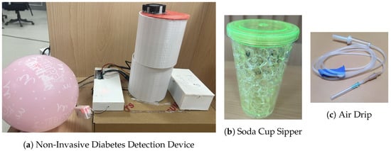
DiabeticSense^[1] (Figure 1a) comprises a sensor array of various MOS-type electrochemical sensors arranged in a cylindrical manner and integrated into a soda sipper cup by tightly closing the cap (Figure 1b). Birthday balloons were used to collect breath samples, and a drip pipe was used to slowly infuse the breath sample into the device (Figure 1c).

4. Details of Sensors Used

To develop the multi-sensor breath analysis device, researchers used an array of sensors that include TGS 822, TGS 826, TGS 2600, TGS 2602, TGS 2603, TGS 2610, TGS 2620, and MQ 138. All the TGS sensors were manufactured by Figaro Inc., Osaka, Japan, while the MQ 138 sensor was manufactured by Zhengzhou Winsen Electronics Technology Co., Ltd., Zhengzhou, China. The sensors that researchers used have sensitivity to a broad range of gases and are not sensitive to any one particular gas. Thus, the sensors are not highly specific to a particular gas. Researchers also used a DHT 22 sensor to record the temperature and humidity while conducting the experiments. DHT 22 is manufactured by the Aosong Electronics Co., Ltd., Guangzhou, China.

• TGS 826: The sensing element of TGS 826 is a metal–oxide–semiconductor that has low conductivity in clean air. In the presence of a detectable gas, the sensor’s conductivity increases depending on the gas concentration in the air. A simple electrical circuit can convert the change in conductivity to an output signal corresponding to the gas concentration. The TGS 826 has sensitivity to VOCs such as iso-butane, ethanol, ammonia, and hydrogen gas. The sensor can detect concentrations as low as 30 ppm in the air and is ideally suited to critical safety-related applications such as the detection of ammonia leaks in refrigeration systems and ammonia detection in the agricultural field ^[5].
• TGS 2610: TGS 2610 is a semiconductor-type gas sensor that combines very high sensitivity to Liquefied petroleum (LP) gas with low power consumption and long life. Due to the miniaturization of its sensing chip, TGS 2610 requires a heater current of only 56 mA and the device is housed in a standard TO-5 package. The TGS 2610 is available in two different models with different external housings but identical sensitivity to LP gas. Both models can satisfy the requirements of performance standards such as UL1484 and EN50194. TGS 2610-C00 possesses a small size and quick gas response, making it suitable for gas leakage checkers. TGS 2610-D00 uses filter material in its housing, eliminating the influence of interference gasses such as alcohol, resulting in a highly selective response to LP gas. This feature makes the sensor ideal for residential gas leakage detectors, which require durability and resistance against interference gas ^[6]. TGS 2610 shows sensitivity to ethanol, hydrogen, methane, iso-butane, and propane gas.
• TGS 822: The sensing element of TGS 822 Figaro gas sensors is a tin dioxide (Sn𝑂₂) semiconductor with low conductivity in clean air. In the presence of a detectable gas, the sensor’s conductivity increases depending on the gas concentration in the air. A simple electrical circuit can convert the change in conductivity to an output signal corresponding to the gas concentration. The TGS 822 is highly sensitive to the vapors of organic solvents and other volatile vapors. It is also sensitive to combustible gasses such as carbon monoxide, making it an excellent general-purpose sensor. It is also available with a ceramic base highly resistant to severe environments as high as 200 °C (in TGS 823). The complete list of gases that TGS 822 is sensitive to include methane, carbon monoxide, iso-butane, n-hexane, benzene, ethanol, and acetone ^[7].
• TGS 2602: The sensing element consists of a metal–oxide–semiconductor layer formed on the alumina substrate of a sensing chip together with an integrated heater. The TGS 2602 is highly sensitive to low concentrations of odorous gasses such as hydrogen, hydrogen sulfide, and ammonia generated from waste materials in office and home environments. The sensor is also susceptible to low concentrations of VOCs, such as toluene and ethanol emitted from wood finishing and construction products. Due to the miniaturization of the sensing chip, TGS 2602 requires a heater current of only 56 mA and the device is housed in a standard TO-5 package ^[8].
• TGS 2600: This sensor is highly sensitive to low concentrations of gaseous air contaminants in cigarette smoke, such as hydrogen, methane, and carbon monoxide, and also shows sensitivity to iso-butane and ethanol. In the presence of a detectable gas, the sensor’s conductivity increases depending on the gas concentration in the air. The sensor can detect hydrogen at a level of several ppm. Due to the miniaturization of the sensing chip, TGS 2600 requires a heater current of only 42 mA and the device is housed in a standard TO-5 package ^[9].
• TGS 2603: The sensing element consists of a metal–oxide–semiconductor layer formed on an alumina substrate of a sensing chip together with an integrated heater. In the presence of a detectable gas, the sensor’s conductivity increases depending on the gas concentration in the air. The TGS 2603 is highly sensitive to low concentrations of odorous gasses such as amine-series and sulfurous odor generated from waste materials or spoiled foods such as fish, such as methyl mercaptan and trimethyl amine, and is also sensitive to hydrogen sulfide, hydrogen, and ethanol. By utilising the change ratio of sensor resistance from the resistance in clean air as the relative response, human perception of air contaminants can be simulated and practical air quality control can be achieved ^[10].
• TGS 2620: The sensing element consists of a metal–oxide–semiconductor layer formed on an alumina substrate of a sensing chip together with an integrated heater. In the presence of a detectable gas, the sensor’s conductivity increases depending on the gas concentration in the air. The TGS 2620 is highly sensitive to the vapors of organic solvents and other volatile vapors, making it suitable for organic vapor detectors/alarms. The complete list of VOCs TGS 2620 senses includes methane, carbon monoxide, iso-butane, hydrogen, and ethanol. Due to the sensing chip’s miniaturization, TGS 2620 requires a heater current of only 42mA and the device is housed in a standard TO-5 package ^[11].
• MQ 138: The sensor measures the change in conductivity of a tin dioxide SnO₂ semiconductor when exposed to VOCs. In clean air, SnO₂ has low conductivity. However, when VOCs are present, they react with the SnO₂ and increase its conductivity. The change in conductivity can be measured as a voltage change, which can then be used to determine the concentration of VOCs in the air. The MQ138 sensor is sensitive to various VOCs, including formaldehyde, benzene, toluene, and acetone. It has a working range of 1 to 100 ppm for benzene ^[12].

• DHT 22: DHT22 is a commonly used temperature and humidity sensor. The sensor has a dedicated NTC thermistor to measure temperature and an 8-bit microcontroller to output temperature and humidity values as serial data. The sensor can measure temperature from −40 °C to 80 °C and humidity from 0% to 100% with an accuracy of ±1 °C and ±1% ^[13].

5. Methodology

Figure 2 illustrates the methodology behind the breath analysis process performed using the device and can be described as follows: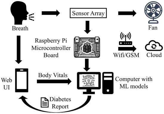

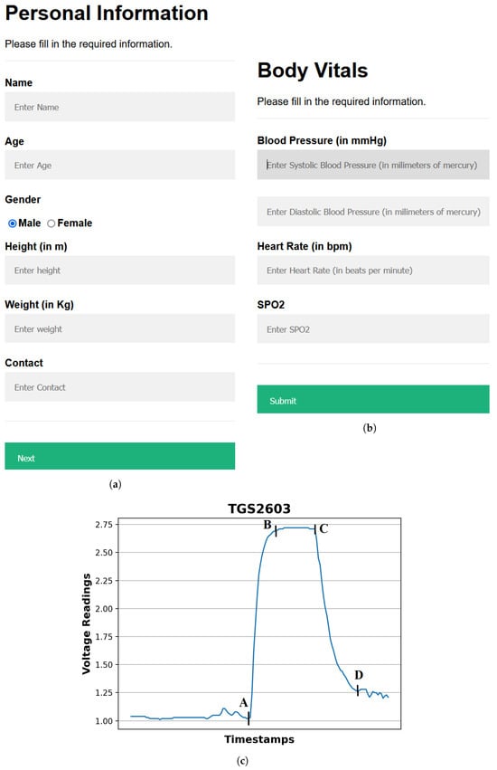
• Providing input details using a web-based interface: The procedure starts by entering the user’s demographic and body vitals information using a web-based interface (Figure 3a,b). The demographics include name, age, gender, height, and weight. To record the body vitals of a user, researchers make them sit in a stable position, rest for five minutes (to make their vitals stable if they have performed some physical activity), and then record their blood pressure, heart rate, and blood oxygen level using standard digital health devices available in the market. These measures can also be self-recorded by a user using digital health devices or a smartwatch and can be entered into the web-based interface. Note: the age recorded in the dataset is when they were detected with diabetes. Furthermore, since most of the T2DM cases occur at ages above 25 years, researchers have currently collected data from patients with an age of more than 25 years ^[14].
• Calibrating the sensors: To ensure accurate sensor readings, researchers calibrate the sensors to establish stable baselines by validating their readings under reference conditions using fresh air. This implies that the sensors were exposed to a known concentration of VOCs and their outputs were recorded. These data can then be used to create a calibration that can be used to correct the sensor readings for any variation. To obtain a stable baseline from the sensor output, the sensors were preheated with a microheater of the gas sensor. Once the sensor’s output stabilizes under fresh-air conditions, breath sample signatures are obtained from the sensor array (details of sensors’ calibration experiments are described in Section 3.5).
• Preheat the sensors: The sensors’ temperature increases to a relatively stable level during use, resulting in a change in the baseline response of the sensors. Therefore, the device was switched on for approximately 20 min until the baseline response shown on the host computer was stable.
• Regular weekly calibration of the sensors: In addition to the initial calibration, researchers also performed regular calibrations every two weeks to reduce the time drift. This is carried out by exposing the sensors to a set of 10 healthy or non-diabetic breath samples and 3 diabetic breath samples, and verifying that the sensor voltages’ range differs for diabetic participants in comparison to the non-diabetic participants. The results of the regular calibrations were used to update the calibration curve, which ensures that the sensor readings remain accurate over time.
• Collecting and infusing the breath sample into the device: A (fasting sugar) breath sample collected in a balloon was infused into the sensor-based setup using a drip pipe mounted on top of the soda cup cap. Researchers placed silica gel packets in a device to absorb moisture (or water) present in breath samples. The drip pipe’s end was attached to the mouth of the inflated balloon, housing the breath sample. The other end was connected to a soda cup cap containing the embedded sensors.
• Processing the breath sample and recording the data: Upon interaction with the VOCs present in the breath sample, the sensors showed deflection from their baseline (as shown in Figure 3c). The recorded deflection data conveyed through the MQTT protocol are directed into an InfluxDB time series database. The Grafana visualization dashboard facilitates the visualization of real-time sensor responses. The experimental setup comprised a Raspberry Pi hosting the MQTT server, Grafana, Node-RED, and Influx DB running as a Docker container. The sensor voltage readings acted as those of characteristics as they depended on the concentration of VOCs in the breath sample.
• Getting the setup ready for the following sample: After a reaction time of two seconds, researchers removed the cup’s cap and mounted it with a fan assembly to expel the breath sample present in the device. Once the voltage readings were restored to their baselines, researchers stopped recording these for the present sample. At this stage, the setup is ready to process the next breath sample.

The sensor voltages collected for each breath sample represent the characteristics of how various sensors sense the VOCs’ concentrations present in the breath sample, and thus collectively represent an instantaneous breath profile of a person. The breath profile may change with time (based on metabolic processes in the body) or due to the consumption of various food items. While collecting the VOC-sensitive sensor data, researchers also recorded the sensors’ readings for temperature and humidity and normalized the sensor voltage readings using the temperature and humidity sensor readings to negate their effect (if any). Such a collection of normalized sensor-based voltage data and the body vitals data obtained by processing various breath samples collectively forms the dataset. Such normalized feature sets and the use of silica packets to absorb moisture during breath sample processing helped to minimize problems like air from the oral cavity and the influence of temperature and humidity. Researchers used the dataset to train and validate various ML models and obtain the best-performing ML model, which was used to generate a diabetes prediction report for a new test breath sample, as shown in Figure 4. As shown in Figure 3c, the sensor voltages are irregular before point A and after point D; segment AB represents the switching state where the sensor starts reacting with the VOCs present in the breath; segment BC represents a stable ON state when the sensor voltages become stable; and the segment CD represents the switching phase when the effect of VOCs starts diminishing. The sensors start coming close to their baseline voltages. DiabeticSense provides instantaneous glucose testing by analyzing the VOCs present in the breath sample at that very instant when submitted for analysis. Also, the user receives an instantaneous response to the test in less than two seconds from the device. Therefore, the testing takes place instantaneously to avoid rapid changes in the concentration of glucose in the blood. Furthermore, researchers collected five samples from all the patients researchers considered while developing the ground truth breath-based sensor voltage dataset to ensure accurate results. Similarly, the user may take three to five instantaneous tests using the device (with a gap of three seconds between each test) to confirm the results and minimize the error.

6. Sensor Calibration Experiments

Since the sensors do not show specificity to specific gases and instead are sensitive to multiple VOCs, researchers did not have the option to calibrate them using specific gases. However, since the objective is to detect diabetic people whose breath contains an increased concentration of acetone, researchers performed bi-fold calibration experiments. First, researchers performed a calibration of the sensors by varying acetone concentrations, i.e., 2, 10, 20, and 40 mL. Specifically, to create a one-part per million (ppm) mixture of acetone, researchers evaporated 2.2302 mL acetone in a 177 m3 dimensions lab and sealed all the openings of the room ^[15]. Similarly, when researchers evaporated 4.4604 mL of acetone in the same room, researchers obtained a 2 ppm acetone mixture. The breath samples collected from this room containing air with a 2 ppm acetone mixture were used for the first set of calibration experiments. The procedure was repeated for calibration with acetone concentrations of 10, 20, and 40 mL. 

7. Clinical Trial Study and Experimental Setting

To evaluate the performance of DiabeticSense, researchers conducted a clinical trial study by collecting the body vitals and breath samples from 110 patients (36 females and 74 males) in a controlled environment at a reputed national hospital. To collect the breath samples of 110 patients, researchers asked the patients to blow out birthday balloons and record their body vitals using standard digital health devices. To establish and develop the ground truth in data (whether a patient was diabetic), researchers collected the blood glucose readings from patients’ clinical blood reports from the hospital from which researchers collected the breath samples. From the collected breath samples, 100 out of 110 breath samples were finalized after data cleaning and preprocessing. The rejected ten samples had some sensor values missing due to lag in reaching the InfluxDB cloud interface. Of these 100 breath samples, 62 were diabetic and 38 were non-diabetic. Researchers deflated the breath sample balloons one by one into the device to obtain the sensor voltages, and then extracted features from the characteristic curve obtained for the sensor voltages of a sample (Figure 3c).

8. Preprocessing the Sensor Voltages

Preprocessing the sensor voltages is performed to remove noisy voltage points and select the relevant ones for feature extraction and ML model development. The sensor voltages at the onset and end of the sample processing, i.e., at points A and D, are irregular (thus are noise) and must be removed. Therefore, for feature extraction and ML model development, for each sensor, researchers sorted the sensor voltages obtained for each breath sample in descending order and took the top 5 sensor voltage readings, which acted as the true representatives of the breath sample analysis between points A and D. The objective here is to capture the sensor voltages for on state represented by the segment AB in Figure 3c. The dataset formed after obtaining the body vitals information and recording the sensor voltages for breath samples collected from 100 finalized breath samples is available at https://zenodo.org/record/8274426 (accessed on 23 September 2023). Note: researchers did not use the sensor voltages directly for ML model training; instead, the features extracted from these sensor voltages and the body vitals data were collectively provided as input for ML model training and testing. Also, researchers considered the top 5 sensor voltages for each breath sample obtained from all sensors.

9. Feature Extraction

For each of the breath samples and its top 5 sensor voltages, researchers extracted various spatial and frequency features such as curve magnitude, slope, first and second derivatives, etc., as mentioned in ^[4]. The features extracted for each breath sample were concatenated as a single feature vector. The complete set of feature vectors obtained by feature extraction from breath samples forms the feature matrix for ML model development. To balance the feature set, researchers experimented with SMOTE (https://imbalanced-learn.org/stable/references/generated/imblearn.over_sampling.SMOTE.html (accessed on 23 September 2023)) and ADASYN (https://imbalanced-learn.org/stable/references/generated/imblearn.over_sampling.ADASYN.html (accessed on 23 September 2023)) techniques, with ADASYN generating the best performance results (discussed in Section 4). Further, researchers scaled the feature set using the MinMaxScalar (https://scikit-learn.org/stable/modules/generated/sklearn.preprocessing.MinMaxScaler.html (accessed on 23 September 2023)) function of Scikit learn (https://scikit-learn.org/ (accessed on 23 September 2023)) to remove the bias toward individual features.

10. ML Model Development

To perform the diabetes prediction task, researchers experimented with the following ten state-of-the-art ML algorithms by training and testing the feature matrix obtained by processing the breath samples, as discussed in the previous subsection. A random 80:20 split of the feature set was performed, whereby 80% of the feature set was deployed for training and 5-fold cross-validation, while the remaining 20% of the feature set was used for testing.

• Gradient Boosting (G-Boost): G-Boost creates a stage-wise model and generalises the model by allowing for the optimization of an arbitrary differentiable loss function. Gradient boosting combines weak learners into a single strong learner in an iterative fashion. As each weak learner is added, a new model is fitted to provide a more accurate estimate of the response variable ^[16][17].
• Decision Tree (DT): A DT is developed by recursively splitting data based on feature values to develop subsets that are as pure as feasible, which means that each subset mainly comprises instances of a single class ^[18].
• K-Nearest Neighbours (KNNs): KNNs do not make any underlying assumptions about data distribution. Given some prior data (training data), KNNs classify coordinates identified by an attribute ^[18].
• Ridge: Ridge regression enhances regular linear regression by slightly changing its cost function, which results in less overfit models ^[19].
• Lasso: Lasso is a regression analysis method that performs both variable selection and regularization to enhance the prediction accuracy and interpretability of the resulting statistical model. For lasso, the coefficient estimates do not need to be unique if covariates are collinear. Lasso’s ability to perform subset selection relies on the form of the constraint and has a variety of interpretations, including in terms of geometry, Bayesian statistics, and convex analysis ^[20][21].
• Elastic Net (ENet): ENet combines the two most popular regularized variants of linear regression: ridge and lasso. Ridge utilises an L2 penalty, and Lasso uses an L1 penalty. ENet uses both the L2 and the L1 penalty ^[22].
• Logistic Regression: It is used for predicting the categorical dependent variable using a given set of independent variables. Logistic regression predicts the output of a categorical dependent variable. Therefore the outcome must be a categorical or discrete value. It can be either yes or no, 0 or 1, true or false, etc., but instead of giving the exact value as 0 and 1, it gives the probabilistic values between 0 and 1 ^[23].
• Support Vector Machines (SVMs): SVMs operate by determining the appropriate hyperplane for separating various classes in the data space. The hyperplane is chosen to maximize the margin, which is the distance between the hyperplane and the nearest data points of each class, also known as support vectors ^[24].
• eXtreme Gradient Boosting (XG-Boost): XG-Boost is an open-source software library with a regularising gradient boosting framework for C++, Java, Python, R, Julia, Perl, and Scala. It works on Linux, Windows, and macOS. From the project description, it aims to provide a scalable, portable and distributed gradient boosting (GBM, GBRT, GBDT) library. It runs on a single machine, and the distributed processing frameworks Apache Hadoop, Apache Spark, Apache Flink, and Dask ^[25].
• Random Forest (RF): The RF algorithm generates multiple DTs during training by selecting random subsets of the original dataset and random subsets of characteristics for each tree. Each DT in the RF is developed using a technique known as recursive partitioning, which involves repeatedly splitting the data into subsets depending on the most discriminatory attributes, resulting in a tree-like structure ^[24].

11. Evaluation Metrics

To obtain the best-performing ML model for the diabetes prediction device, researchers compared the performance of various ML models trained on the dataset using the evaluation metrics described as follows: researchers selected Accuracy (https://scikit-learn.org/stable/modules/generated/sklearn.metrics.accuracy_score.html (accessed on 23 September 2023)), F1 Score (http://scikit-learn.org/stable/modules/generated/sklearn.metrics.f1_score.html (accessed on 23 September 2023)) and ROC curve area (http://scikit-learn.org/stable/auto_examples/model_selection/plot_roc.html (accessed on 23 September 2023)) metrics as the evaluation metrics of the work, defined as follows: where and Because the F1 score captures both the effect of Precision and Recall, researchers computed the F1 Score values and their respective standard deviation values (or error values) only. The higher the F1 Score, the better the model’s prediction accuracy. ROC Area Under the Curve (AUC) metric evaluates the output quality. A ROC curve is a plot that features the true positive rate. (marked as the Y-axis) versus the false positive rate (marked as the X-axis) for an experiment. The point at the top-left corner of the plot depicts the point of the most ‘ideal’ behavior having the {false positive rate, true positive rate} pair value as {0, 1}. Thus, a larger area under the curve signifies a better quality output. researchers therefore selected the ROC curve area as the second evaluation metric. Since the highest Accuracy value, F1 Score value, and ROC AUC value may differ across the models, researchers took the average of these metrics as the final accuracy measure of a model (MeanAcc defined in Equation (5)).

12. Selecting the Best-Performing Model for Diabetes Prediction

Since researchers used multiple evaluation metrics to compare the performance of these ML models, researchers selected the best-performing model by taking an average (or mean) of the performance metrics for each of the ML models, described in detail as follows: Researchers define the best-performing ML model as the one with the highest MeanAcc measure value, where MeanAcc is represented by Equation (5). There, A represents the set of ML algorithms and Π is the tuning parameter combinations set, such that Δ𝛼,𝜋 represents the ML model built using the ML algorithm 𝛼 with the parameter combination 𝜋, such that 𝛼∈𝐴,𝑎𝑛𝑑𝜋∈Π. The complete list of ML algorithms (A) and the hyper-tuning parameters used (Π) is found. As shown in Equation (5) above, MeanAcc is computed simply by performing an average of F1 Score, Accuracy, and ROC AUC metrics values obtained by using the best hyper-tuned parameter values. Thus, the problem of finding the best-performing model trained on the dataset (containing sensor and body vital readings) to perform the diabetes prediction for a test breath sample can be defined as follows: