Your browser does not fully support modern features. Please upgrade for a smoother experience.
Please note this is a comparison between Version 1 by Guang Lin and Version 2 by Catherine Yang.
Non-dominated sorting genetic algorithm (NSGA)-Physics-informed neural networks (PINNs), a multi-objective optimization framework for the effective training of PINNs.
- machine learning
- data-driven scientific computing
- multi-objective optimization
1. Introduction
Physics-informed neural networks (PINNs) [1][2][1,2] have proven to be successful in solving partial differential equations (PDEs) in various fields, including applied mathematics [3], physics [4], and engineering systems [5][6][7][5,6,7]. For example, PINNs have been utilized for solving Reynolds-averaged Navier–Stokes (RANS) simulations [8] and inverse problems related to three-dimensional wake flows, supersonic flows, and biomedical flows [9]. PINNs have been especially helpful in solving PDEs that contain significant nonlinearities, convection dominance, or shocks, which can be challenging to solve using traditional numerical methods [10]. The universal approximation capabilities of neural networks [11] have enabled PINNs to approach exact solutions and satisfy initial or boundary conditions of PDEs, leading to their success in solving PDE-based problems. Moreover, PINNs have successfully handled difficult inverse problems [12][13][12,13] by combining them with data (i.e., scattered measurements of the states).
PINNs use multiple loss functions, including residual loss, initial loss, boundary loss, and, if necessary, data loss for inverse problems. The most common approach for training PINNs is to optimize the total loss (i.e., the weighted sum of the loss functions) using standard stochastic gradient descent (SGD) methods [14][15][14,15], such as ADAM. However, optimizing highly non-convex loss functions for PINN training with SGD methods can be challenging because there is a risk of being trapped in various suboptimal local minima, especially when solving inverse problems or dealing with noisy data [16][17][16,17]. Additionally, SGD can only satisfy initial and boundary conditions as soft constraints, which may limit the use of PINNs in the optimization and control of complex systems, which require the exact fulfillment of these constraints.
2. The NSGA-PINN Framework
This section describes the proposed NSGA-PINN framework for multi-objective optimization-based training of a PINN.2.1. Non-Dominated Sorting
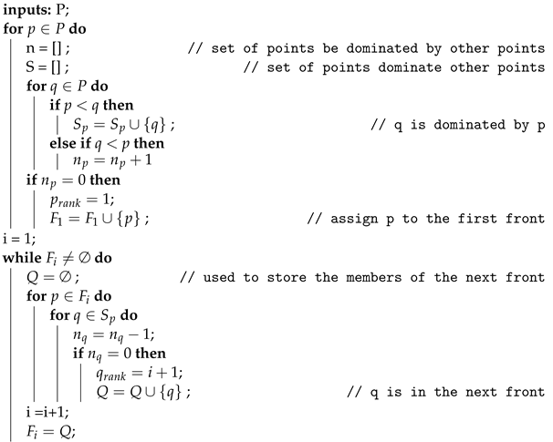
The proposed NSGA-PINN utilizes non-dominated sorting (see Algorithm 1 for more detailed information) during PINN training. The input P can consist of multiple objective functions, or loss functions, depending on the problem setting. For a simple ODE problem, these objective functions may include a residual loss function, an initial loss function, and a data loss function (if experimental data are available and thwe researchers are are tackling an inverse problem). Similarly, for a PDE problem, the objective functions may include a residual loss function, a boundary loss function, and a data loss function. In the EAs, the solutions refer to the elements in the parent population. ThWe researchers raandomly choose two solutions in the parent population p and q; if p has a lower loss value than q in all the objective functions, thwe researchers define p as dominating q. If p has at least one loss value lower than q, and all others are equal, the previous definition also applies. For each p element in the parent population, thwe researchers ccalculate two entities: (1) domination count 𝑛𝑝, which represents the number of solutions that dominate solution p, and (2) 𝑆𝑝, the set of solutions that solution p dominates. Solutions with a domination count of 𝑛𝑝=0 are considered to be in the first front. ThWe researchers then look at 𝑆𝑝 and, for each solution in it, decrease their domination count by 1. The solutions with a domination count of 0 are considered to be in the second front. By performing the non-dominated sorting algorithm, thwe researchers obtain the front value for each solution [18][21].| Algorithm 1: Non-dominated sorting |
 |
2.2. Crowding-Distance Calculation
In addition to achieving convergence to the Pareto-optimal set for multi-objective optimization problems, it is important for an evolutionary algorithm (EA) to maintain a diverse range of solutions within the obtained set. ThWe researchers implement the crowding-distance calculation method to estimate the density of each solution in the population. To do this, first, sort the population according to each objective function value in ascending order. Then, for each objective function, assign infinite distance values to the boundary solutions, and assign all other intermediate solutions a distance equal to the absolute normalized difference in function values between two adjacent solutions. The overall crowding-distance value is calculated as the sum of individual distance values corresponding to each objective. A higher density value represents a solution that is far away from other solutions in the population.2.3. Crowded Binary Tournament Selection
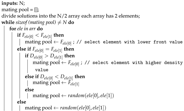
The crowded binary tournament selection, explained in more detail in Algorithm 2, was used to select the best PINN models for the mating pool and further operations. Before implementing this selection method, thwe researchers labeled each PINN model so that the researchers cwe could track the one with the lower loss value. The population of size n was then randomly divided into 𝑛/2 groups, each containing two elements. For each group, thwe researchers ccompared the two elements based on their front and density values. The researchers We preferred the element with a lower front value and a higher density value. In Algorithm 2, F denotes the front value and D denotes the density value.| Algorithm 2: Crowded binary tournament selection |
 |
| Algorithm 2: Crowded binary tournament selection |
 |
2.4. NSGA-PINN Main Loop
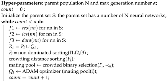
The main loop of the proposed NSGA-PINN method is described in Algorithm 3. The algorithm first initializes the number of PINNs to be used (N) and sets the maximum number of generations (𝛼) to terminate the algorithm. Then, the PINN pool is created with N PINNs. For each loss function in a PINN, N loss values are obtained from the network pool. When there are three loss functions in a PINN, 3𝑁 loss values are used as the parent population. The population is sorted based on non-domination, and each solution is assigned a fitness (or rank) equal to its non-domination level [18][21]. The density of each solution is estimated using crowding-distance sorting. Then, by performing a crowded binary tournament selection, PINNs with lower front values and higher density values are selected to be put into the mating pool. In the mating pool, the ADAM optimizer is used to further reduce the loss value. The NSGA-II algorithm selects the PINN with the lowest loss value as the starting point for the ADAM optimizer. By repeating this process many times, the proposed method helps the ADAM optimizer escape the local minima. Figure 12 shows the main process of the proposed NSGA-PINN framework.| Algorithm 3: Training PINN by NSGA-PINN method |
 |
| Algorithm 3: Training PINN by NSGA-PINN method |
 |
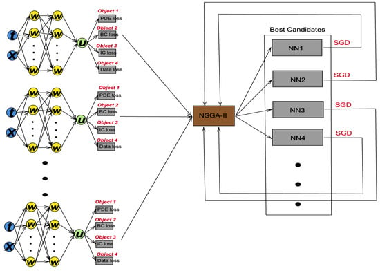
Figure 12. NSGA-PINN structure diagram.
