Your browser does not fully support modern features. Please upgrade for a smoother experience.
Please note this is a comparison between Version 1 by Konstantinos Karampidis and Version 2 by Catherine Yang.
The field of brain–computer interface (BCI) enables us to establish a pathway between the human brain and computers, with applications in the medical and nonmedical field. Brain computer interfaces can have a significant impact on the way humans interact with machines. In recent years, the surge in computational power has enabled deep learning algorithms to act as a robust avenue for leveraging BCIs.
- EEG
- deep learning
- BCI
- motor imagery
1. Introduction
Brain–computer interfaces (BCIs) are an emerging field of technology that combines and allows the connection between the brain and a computer or other external devices. BCIs have the potential to revolutionize the way humans interact with machines, opening countless possibilities both in medical and nonmedical domains. In the medical field, it can help people suffering from locked-in syndrome to communicate [1]. Moreover, brain–computer interfaces (BCIs) are displaying potential in the realm of neuroprosthetics, offering the prospect for individuals with limb amputations or paralysis to command robotic limbs or exoskeletons through their brain signals [2]. In epilepsy management, BCIs are researched for real-time seizure detection and intervention, potentially mitigating the impacts of seizures [3]. In the nonmedical domain, an EEG BCI has applications in areas such as gaming where players can play a game using only their thoughts [4] and in fields such as entertainment where users can control drones or other robotic devices [5].
2. Convolutional Neural Networks
CNNs mimic the operational principles of the human visual cortex and possess the ability to dynamically comprehend spatial hierarchies in EEG data, recognizing patterns associated with motor imagery tasks through multiple layer transformations [6][51]. A CNN architecture begins with an input layer that accepts raw or preprocessed EEG data as shown in Figure 19. These data can be represented in various formats, such as time–frequency images, allowing the network to effectively process and analyze the brain signals associated with motor imagery. These data are then convolved using multiple kernels or filters, enabling the network to learn local features. Subsequently, the network employs a pooling layer for dimensionality reduction, refining the comprehension of the information. As the model progresses through these layers, it acquires the capacity to understand increasingly complex features. The final component is a fully connected (dense) classification layer that maps the learned high-level features to the desired output classes, such as different types of motor imagery, effectively acting as a decision-making layer that converts abstract representations into definitive classifications. Dose et al. proposed a CNN trained on 3 s of segments from EEG signals [8][53]. The proposed method achieved an accuracy of 80.10%, 69.72%, and 59.71% on two, three, and four MI classes, respectively, on the Physionet dataset. Miao M et al. proposed a CNN with five layers to classify two motor imagery tasks, right hand and right foot, from the BCI Competition III-IV-a dataset, achieving a 90% accuracy [9][54]. Zhao et al. proposed a novel CNN with multiple spatial temporal convolution (STC) blocks and fully connected layers [10][55]. Contrastive learning was used to push the negative samples away and pull the positive samples together. This method achieved an accuracy of 74.10% on BCI III-2a, 73.62% on SMR-BCI, and 69.43% on OpenBMI datasets. Liu et al. proposed an end-to-end compact multibranch one-dimensional CNN (CMO-CNN) network for decoding MI EEG signals, achieving 83.92% and 87.19% accuracies on the BCI Competition IV-2a and the BCI Competition IV-2b datasets, respectively [11][56]. Han et al. proposed a parallel CNN (PCNN) to classify motor imagery signals [12][57]. That method, which achieved an average accuracy of 83.0% on the BCI Competition IV-2b dataset, began by projecting raw EEG signals into a low-dimensional space using a regularized common spatial pattern (RCSP) to enhance class distinctions. Then, the short-time Fourier transform (STFT) collected the mu and beta bands as frequency features, combining them to form 2D images for the PCNN input. The efficacy of the PCNN structure was evaluated against other methods such as stacked autoencoder (SAE), CNN-SAE, and CNN. Ma et al. proposed an end-to-end, shallow, and lightweight CNN framework, known as Channel-Mixing-ConvNet, aimed at improving the decoding accuracy of the EEG-Motor Raw datasets [13][58]. Unlike traditional methods, the first block of the network was designed to implicitly stack temporal–spatial convolution layers to learn temporal and spatial EEG features after EEG channels were mixed. This approach integrated the feature extraction capabilities of both layers and enhanced performance. This resulted in a 74.9% accuracy rate on the BCI IV-2a dataset and 95.0% accuracy rate on the High Gamma Dataset (HGD). Ak et al. performed an EEG data analysis to control a robotic arm. In their work, spectrogram images derived from EEG data were used as input to the GoogLeNet. They tested the system on imagined directional movements—up, down, left, and right—to control the robotic arm [14][59]. The approach resulted in the robotic arm executing the desired movements with over 90% accuracy, while on their private dataset, they achieved 92.59% accuracy. Musallam Y et al. proposed the TCNet-Fusion model, which used multiple techniques such as temporal convolutional networks (TCNs), separable convolution, depthwise convolution, and layer fusion [15][60]. This process created an imagelike representation, which was then fed into the primary TCN. During testing, the model achieved a classification accuracy of 83.73% on the four-class motor imagery of the BCI Competition IV-2a dataset and an accuracy of 94.41% on the High Gamma Dataset. Zhang et al. proposed a CNN with a 1D convolution on each channel followed by a 2D convolution to extract spatial features based on all 20 channels [16][61]. Then, to deal with the high computational cost, the idea of pruning was used, which is a technique of reducing the size and complexity of the neural network by removing certain connections or neurons. In the proposed method, a fast recursive algorithm (FRA) was applied to prune redundant parameters in the fully connected layers to reduce computational costs. The proposed architecture achieved an accuracy of 62.7% in the OPENBCI dataset. A similar approach was proposed by Vishnupriya et al. [17][62] to reduce the complexity of their architecture. The magnitude-based weight pruning was performed on the network, which achieved an accuracy of 84.46% on two MI tasks (left hand, right hand) in Lee et al.’s dataset. Shajil et al. proposed a CNN architecture to classify four MI tasks, using the common spatial pattern filter on the raw EEG signal, then using the spectrograms extracted from the filtered signals as input into the CNN [18][63]. The proposed method achieved an accuracy of 86.41% on their private dataset. Korhan et al. proposed a CNN architecture with five layers [19][64]. The proposed architecture was compared using only the CNN without any filtering, then with five different filters, and finally, with common spatial patterns followed by the CNN with the last architecture, which achieved the highest accuracy of 93.75% in the BCI Competition III-3a dataset. Alazrai et al. proposed a CNN network, with the raw signal transformed into the time–frequency domain with the quadratic time–frequency distribution (QTFD), followed by the CNN network to extract and classify the features [20][65]. The proposed method was tested on their two private datasets, with 11 MI tasks (rest, grasp-related tasks, wrist-related tasks, and finger-related tasks) and obtained accuracies of 73.7% for the able-bodied and 72.8% for the transradial-amputated subjects. Table 12 summarizes the research articles that utilize CNNs along with the tasks, the datasets used, and their performance.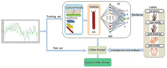
Table 12.
Reviewed CNN architectures, datasets and their accuracies.
Table 34.
Reviewed deep neural network architectures and their accuracies.
| Authors | Accuracy | Dataset | MI Tasks | ||||
|---|---|---|---|---|---|---|---|
| Suhaimi et al. [35][79] | 49.5% | BCI Competition 2b | LH, RH | ||||
| Wei et al. [25][70] | 81.8%, 54.8% | BCI IV-2a, private | LH, RH | ||||
| Zhao R et al. [ | |||||||
| Cheng et al. [36][80] | 71.5% | Private | LH, RH | 10][55] | 74.10%, 73.62%, 69.43% | BCI III-2a, SMR-BCI, OpenBMI | RH, RF |
| Liu X et al. [11][56] | 83.92%, 87.19% | BCI IV-2a, BCI IV-2b | LH, RH, BL, T |
.
Table 45.
Other reviewed deep learning architectures and their accuracies.
| Authors | Accuracy | Dataset | MI Tasks | Architecture | ||
|---|---|---|---|---|---|---|
| Autthasan et al. [41][85] | 70.09%, 72.95% 66.51% |
BCI IV-2a, SMR_BCI, Open BCI | LH, RH, BL, T | Autoencoder | ||
| Ha et al. [43][87] | 77% | BCI IV-2b | ||||
| Limpiti et al. [29][73] | 95.03%, 91.86% | BCI IV-2a | LH, RH, BL, T | |||
| LH, RH | Capsule network | Yohonanndan et al. [37][81] | 83% | Private | RS, RH | |
| Urbano et al. [45][89] | 90% | MNE dataset | Han et al. [12][57] | 83% | BCI IV-2b | LH, RH |
| Ma et al. [13][58] | 74.9%, 95.0% | BCI IV-2a, HGD | LH, RH, BL, T | |||
| Ak et al. [14][59] | 92.59% | Private | U, D, L, R | |||
| Musallam et al. [15][60] | 83.73%, 94.41% | BCI IV-2a, HGD | LH, RH, BL, T | |||
| Zhang et al. [16][61] | 62.7% | OpenBMI | LH, RH | |||
| Vishnupriya et al. [17][62] | 84.46% | Lee et al. | LH, RH | |||
| Shajil et al. [18][63] | 86.41% | Private | LH, RH, BH, BL | |||
| Korhan et al. [19][64] | 93.75% | BCI III-3a | LH, RH, BL, T | |||
| Alazrai et al. [20][65] | 73.7%, 72.8% | Private | RS, SDG, LG, ETG, RDW, EW, FI, FM, FR, FL, FT |
LH: left hand, RH: right hand, RL: right leg, BL: both legs, T: tongue, RS: resting state, BF: Both fists, LF: left fist, RF: right fist, U: up, D: down, L: left, R: right, SDG: small-diameter grasp, LG: lateral grasp, ETG: extension-type grasp, RDW: ulnar and radial deviation of the wrist, EW: extension of the wrist, FI: flexion and extension of the index finger, FM: flexion and extension of the middle finger, FR: flexion and extension of the ring finger, FL: flexion and extension of the little finger.
3. Transfer Learning
In the realm of machine learning, transfer learning offers a valuable approach to improve model performance and efficiency. It involves leveraging the knowledge learned from one task and applying it to a different but related task. The foundation of transfer learning lies in pretrained models, which have been trained on large-scale datasets. This approach is beneficial when considering the computational resources required for training deep learning models from scratch, i.e., time, complexity, and hardware. Transfer learning also offers a noble solution when available training data are not enough to train effectively novel deep learning models. In these situations, where collecting training data is hard or expensive, as in the case of EEG data, a need to develop robust models using available data from diverse domains arises. However, the effectiveness of transfer learning relies on the learned features from the initial task being general and applicable to the target task. Some popular deep learning models utilized for transfer learning are AlexNet [21][66], ResNet18 [22][67], ResNet50, InceptionV3 [23][68], and ShuffleNet [24][69]. These models are CNN networks trained on millions of images to classify different classes. For example, AlexNet consists of eight layers with weights, the first five are convolutional layers followed by max-pooling layers, and the last three layers are fully connected layers followed by a softmax layer to provide a probability distribution over the 1000 class labels. Figure 210 shows the architecture of the AlexNet architecture. ResNet (residual network) is a deep learning model in which the weight layers learn residual functions with reference to the layer inputs. This method addresses the problem of vanishing gradients in deep neural networks by introducing skip connections, also known as residual blocks. The information can flow directly across multiple layers, making it easier for the network to learn complex features. There are various versions of ResNet utilized for EEG classification, e.g., ResNet34, ResNet50, etc. Figure 311 shows the architecture of ResNet. While some research papers rely on pretrained models for transfer learning, others take a different approach. Let N be the total number of subjects in a dataset. Researchers train a custom CNN on N–1 subjects, and afterwards, they use the trained CNN as a base model for transfer learning. That is, they use the remaining N subject to train the aforementioned CNN, and afterwards, they finetune the whole model. Moreover, some research papers ([25][26][70,71]) opt for alternative architectures, such as the one proposed by Schirrmeister et al. [27][43], to facilitate transfer learning in their studies. Zhang et al. utilized transfer learning to train a hybrid deep neural network (HDNN-TL) which consisted of a convolutional neural network and a long short-term memory model, to decode the spatial and temporal features of the MI signal simultaneously [28][72]. The classification performance on the BCI Competition IV-2a dataset by the proposed HDNN-TL in terms of kappa value was 0.8 (outperforming the rest of the examined methods). Wei et al. [25][70] proposed a multibranch deep transfer network, the Separate-Common-Separate Network (SCSN) based on splitting the network’s feature extractors for individual subjects, and they also explored the possibility of applying maximum mean discrepancy (MMD) to the SCSN (SCSN-MMD). They tested their models on the BCI Competition IV-2a dataset and their own online recorded dataset, which consisted of five subjects (male) and four motor imageries (relaxing, left hand, right hand, and both feet). The results showed that the proposed SCSN achieved an accuracy of (81.8%, 53.2%) and SCSN-MMD achieved an accuracy of (81.8%, 54.8%). Limpiti et al. used a continuous wavelet transform (CWT) to construct the scalograms from the raw signal, which served as input to five pretrained networks (AlexNet, ResNet18, ResNet50, InceptionV3, and ShuffleNet) [29][73]. The models were evaluated on the BCI Competition IV-2a dataset. On binary (left hand vs. right hand) and four-class (left hand, right hand, both feet, and tongue) classification, the ResNet18 network achieved the best accuracies at 95.03% and 91.86%. Wei et al. [30][74] utilized a CWT to convert the one-dimensional EEG signal into a two-dimensional time–frequency amplitude representation as the input of a pre-trained AlexNet and fine-tuned it to classify two types of MI signals (left hand and right hand). The proposed method achieved a 93.43% accuracy on the BCI Competition II-3 dataset. Arunabha proposed a multiscale feature-fused CNN (MSFFCNN) efficient transfer learning (TL) and four different variations of the model including subject-specific, subject-independent, and subject-adaptive classification models to exploit the full learning capacity of the classifier [31][75]. The proposed method achieved a 94.06% accuracy on for four different MI classes (i.e., left hand, right hand, feet, and tongue) on the BCI Competition IV-2a dataset. Chen et al. proposed a subject-weighted adaptive transfer learning method in conjunction with MLP and CNN classifiers, achieving an accuracy of 96% on their own recorded private dataset [32][76]. Zhang et al. proposed five schemes for the adaptation of a CNN to two-class motor imagery (left hand, right hand), and after fine-tuning their architecture, they achieved an accuracy of 84.19% on the public GigaDB dataset [26][71]. Solorzano et al. proposed a method based on transfer learning in neural networks to classify the signals of multiple persons at a time [33][77]. The resulting neural network classifier achieved a classification accuracy of 73% on the evaluation sessions of four subjects at a time and 74% on three at a time on the BCI Competition IV-2a dataset. Li et al. proposed a cross-channel specific–mutual feature transfer learning (CCSM-FT) network model with training tricks used to maximize the distinction between the two kinds of features [34][78]. The proposed method achieved an 80.26% accuracy on the BCI Competition IV-2a dataset. A summary of the aforementioned methods can be found in Table 23.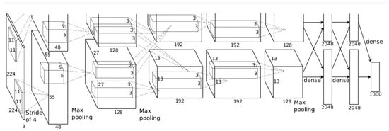
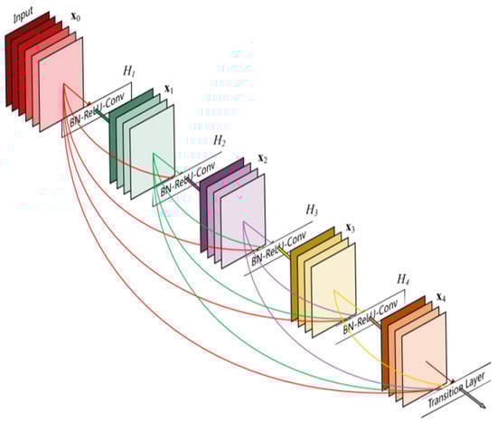
Table 23.
Reviewed transfer learning architectures and their accuracies.
| Authors | Accuracy | Dataset | MI Tasks | |||||
|---|---|---|---|---|---|---|---|---|
| Zang et al. | ||||||||
| BF, BH | ||||||||
| LSTM | ||||||||
| Wei M et al. [30][74] | 93.43% | BCI II-3 | LH, RH | |||||
| Kumar et al. [38][82] | ~85% | BCI Competition III-4a | RH, LF | |||||
| Saputra et al. [46][90] | 49.65% | BCI IV-2a | LH, RH, BL, T | LSTM | Arunabha M. [31][75] | 94.06% | BCI IV-2a | LH, RH, BL, T |
| Hwang et al. [47][91] | 97% | BCI IV-2a | LH, RH, BL, T | LSTM | Chen et al. [32][76] | |||
| Ma et al. [48][92] | 96% | Private | F, B, L, R, S | |||||
| Zhang et al. [26][71] | 84.19% | GigaDB | LH, RH | |||||
| Solorzano et al. [33][77] | 74% | BCI IV-2a | LH, RH, BL, T | |||||
| Li D et al. [34][78] | 80.26% | BCI IV-2a | LH, RH, BL, T |
LH: left hand, RH: right hand, RL: right leg, BL: both legs, T: tongue, RS: resting state, BF: Both fists, LF: left fist, RF: right fist, F: forward, B: backward, L: left, R: right, R: rest, S: stop.
4. Deep Neural Networks
Deep neural networks, a subset of artificial neural networks, have the ability to tackle complex problems. Unlike shallow neural networks that consist of only a few layers, deep neural networks are characterized by their depth, featuring multiple hidden layers between the input and output layers. Each hidden layer progressively extracts higher-level features from the data, allowing the network to learn complex representations and patterns from vast quantities of data. Suhaimi et al. [35][LH: left hand, RH: right hand, LF: left foot, RS: resting state.
5. Others
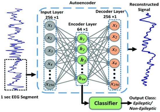
Several alternative methods have been proposed for classifying motor imagery (MI) tasks, aiming at leveraging the potential of different deep learning techniques. Autoencoders [39][83], which are designed for data reconstruction, have been explored in the context of MI task classification. Autoencoders are neural network architectures that consist of two main phases: encoding and decoding. During the encoding phase, the input signal is passed through a neural network with a progressively reduced number of neurons in each layer until it reaches the bottleneck layer, which has a lower dimensionality compared to the input data. In the decoding phase, the network strives to reconstruct the original signal from this lower-dimensional representation, preserving essential information. This encoding stage in autoencoders enables them to effectively learn compressed representations of input data, such as EEG data, by reducing its dimensionality while retaining significant information. Figure 412 shows an autoencoder used to reconstruct an EEG signal.| 68.20% | ||||
| EEGMMIDB | ||||
| LF, RF, BL, BF | ||||
| LSTM, bi-LSTM | ||||
| Xu et al. [50][94] | 78.50% | BCI IV-2a | LH, RH, BL, T | Boltzmann Machine |
| Li et al. [52][96] | 80% | EEGMMIDB | LF, RF, BL, BF | Meta-learning |
| Han et al. [54][98] | 79.54% | BCI IV-2a | LH, RH, BL, T | Contrastive learning |
| Li et al. [56][100] | 93.57% | BCI II-3 | LH, RH | Deep belief network |
LH: left hand, RH: right hand, RL: right leg, BL: both legs, T: tongue, RS: resting state, BF: both fists, LF: left fist, RF: right fist.