Your browser does not fully support modern features. Please upgrade for a smoother experience.
Please note this is a comparison between Version 1 by Xiaobo Li and Version 2 by Rita Xu.
Traditional lidar techniques mainly rely on the backscattering/echo light intensity and spectrum as information sources. In contrast, polarization lidar (P-lidar) expands the dimensions of detection by utilizing the physical property of polarization. By incorporating parameters such as polarization degree, polarization angle, and ellipticity, P-lidar enhances the richness of physical information obtained from target objects, providing advantages for subsequent information analysis.
- polarization
- lidar
- remote sensing
- P-lidar
1. Introduction
Polarization, akin to parameters such as frequency, phase, and amplitude/intensity, represents a fundamental physical property of light [1][2][3][1,2,3]. The earliest records of polarized light can be traced back to 1669, when Bartholin discovered the phenomenon of double-refraction in a piece of Iceland spar (calcite), which paved the way for human exploration of polarized optics [2]. Subsequently, in 1678, Huygens proposed the wave theory of light, providing a satisfactory explanation for the polarization characteristics of light [2]. Therefore, Huygens is recognized as the first scientist in the history of physics to discover the properties of polarized light.
Polarized light is prevalent in the natural world, primarily resulting from reflection and scattering processes. This is because reflection and scattering often induce varying optical efficiencies and/or phase changes for the orthogonal polarization components of the incident light [3][4][3,4]. Consequently, differences in the surface structure and texture of an object can influence the polarization state of reflected and/or scattered light [5][6][5,6]. By measuring the polarization characteristics of reflected or scattered light, the analysis of surface morphology information becomes possible, leading to extensive applications of polarized light in remote sensing [7][8][7,8]. For example, in passive remote sensing, the polarization characteristics of solar spectral lines serve as important carriers for navigation [9][10][9,10]; when sunlight interacts with water vapor, ice crystals, dust, sand, smoke, and other substances, polarized light can be generated, proving the physical properties of such materials [11][12][11,12]. Furthermore, polarized light plays a significant role in areas including resource exploration, vegetation and soil classification, research on the sea surface, and global atmospheric aerosol studies [5][13][5,13]. In active remote sensing, polarized light is indispensable for detecting aerosols’ shape, identifying cloud phases, and determining particles’ orientation [14][15][16][14,15,16].
In 1916, Einstein proposed the theory of light’s stimulated emission (LSE) [17], which guided humanity to recognize such light with a precise single color and wavelength, which is also named light amplification by stimulated emissions of radiation (laser) [18]. However, it was not until 1960 that the first laser generator was developed, marking the beginning of laser utilization [19]. Actually, the idea of using a laser in radar systems, i.e., light detection and ranging (Lidar), was immediately considered after the laser’s invention [20]. For instance, in 1969, an American team installed a retro-reflector device similar to a mirror on the lunar surface. Laser beams were directed towards this device from Earth, enabling accurate measurement of the Earth–Moon distance [21][22][21,22]. However, lasers quickly expanded beyond this application and found widespread utility in various fields, including surveying, atmospheric remote sensing, and oceanic remote sensing.
Lidar systems consist of three main components: transmitter, receiver, and processing. The transmitter emits a laser beam into a target scene, initiating an interaction between the laser and the target object (such as suspended particles in the atmosphere or seawater), which causes changes in various aspects of the optical signal, including propagation direction, intensity, frequency, polarization, and phase [23]. By detecting these changes and combining transmission models, information related to the target’s physical properties, such as its position, velocity, and composition, can be inferred [24][25][24,25]. Figure 1 presents the basic elements of lidar: the laser sources, ranging principles, beam modulations, and detectors.
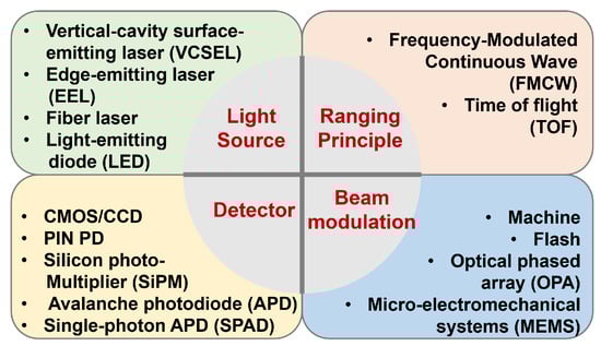
Figure 1. Basic components of lidar.
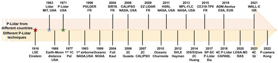
Figure 2. History of P-lidar. 1C: single-channel; 2C: dual-channel; 4C: four-channel; SP: single-photon; other abbreviations can be found in the main text.
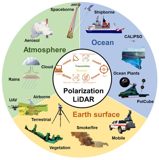
Figure 3. Triad of applications of P-lidar.
2. Applications
2.1. Atmospheric Remote Sensing
Lidar and polarimeter technologies complement each other effectively. Lidar excels at detailing aerosol profiles and types, while polarimeters offer constraints on overall aerosol abundance, absorption, and microphysical properties [13][63][13,101]. Combining these methods enhances aerosol property observations; this is also why P-lidar has been widely employed in atmospheric remote sensing to study the optical properties of the atmosphere and the characteristics of particles such as aerosols, clouds, and water vapor. Specifically, P-lidar can measure the polarization scattering characteristics of aerosol particles, providing information about aerosol concentration, size distribution, shape, etc. This is crucial for understanding aerosol sources, transport, and interaction mechanisms in the atmosphere. By measuring polarization scattering properties using P-lidar, information such as aerosol types, cloud optical thickness, particle size, and shape distribution can be obtained.
This is significant for studying cloud formation and evolution and their impact on climate and weather. P-lidar can measure atmospheric transparency parameters such as atmospheric optical thickness and aerosol optical depth. This is important for monitoring atmospheric pollution and studying atmospheric composition [14][64][14,49].
In 1963, the Massachusetts Institute of Technology (MIT) established the first lidar based on ruby lasers, which was used to detect high-altitude aerosols in the troposphere and middle atmosphere [65][123]. This marked the beginning of the development and application of lidar for aerosol detection. Around the same time, mature polarization optical techniques were applied to lidar systems. In the 1960s, New York University began using polarization lidar, i.e., P-lidar, systems to observe atmospheric ice crystals and water droplets [39]. As shown in Figure 4, ice crystal detection hinges on measuring the volume depolarization ratio. While backscattering from spherical objects (such as liquid drops) at exactly 180∘ yields no depolarization, non-spherical crystal backscattering introduces notable depolarization through multiple internal reflections. Thus, the volume depolarization ratio effectively distinguishes between cloud layers with water drops and those where backscattering by ice crystals prevails [66][124]. In 1971, Schotland et al. conducted research on the depolarization ratio of water vapor condensates [39]. Understanding and quantifying the various forms of ice crystals in the atmosphere and precipitation are crucial for comprehending microphysical and radiative processes in different scenarios and improving regional and global climate models. In 2017, Sergey et al. used measurements from the U.S. Department of Energy’s Atmospheric Radiation Measurement (ARM) program’s cloud P-lidar to retrieve the nonsphericity of ice particles. The observed ice particles included irregularly shaped crystals and aggregates, with aspect ratios spanning from around 0.3 to 0.8 [67][125].
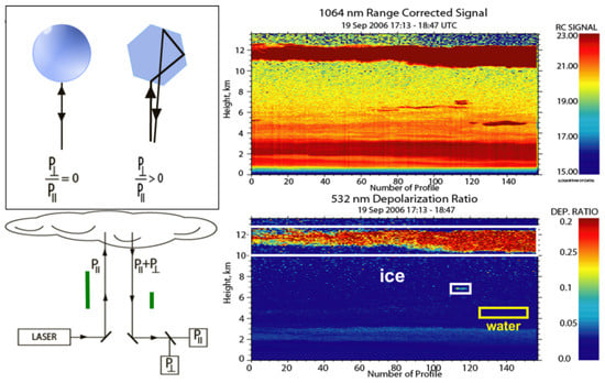
Figure 4. Demonstration of P-lidar for distinguishing liquid cloud droplets and ice crystals.
Using polarization information for particle shape measurement and properties’ analysis is a well-established technique. In 2015, Wu et al. developed the Water Vapor, Cloud, and Aerosol Lidar (WACAL) for comprehensive atmospheric measurements, including the water vapor mixing ratio, depolarization ratio, backscatter and extinction coefficients, and cloud information [68][126]. The WACAL system, featuring Raman, polarization, and infrared channels, was installed at Qingdao Ocean University, enabling the assessment of aerosol and cloud optical properties and water vapor mixing ratios. In 2019, Tan et al. introduced a novel method to infer the phase state of submicron particles using linear depolarization ratios obtained from P-lidar [69][127]. This innovative approach demonstrated the feasibility of inferring aerosol phase distributions and established a parameterization scheme for deducing aerosol phase states from backscatter depolarization ratios, marking a significant advancement in real-time aerosol phase state profiling. In 2020, Jimenez et al. first introduced a novel cloud-retrieval technique using lidar observations of the volume linear depolarization ratio at two different receiver field of views (FOVs) to retrieve the micro-physical properties of liquid cloud layers [70][128] and then applied it to cloud measurements in pristine marine conditions at Punta Arenas in southern Chile [71][129]. Following Jimenez’s work, in 2023, Zhang et al. introduced a dual-FOV high-spectral-resolution Lidar (HSRL) for simultaneous analysis of aerosol and water cloud properties, particularly the microphysical properties of liquid water clouds. This instrument allowed for continuous monitoring of aerosols and clouds and underwent validation through synchronous observations, including Monte Carlo simulations and other methods, to investigate the interplay between aerosol levels and the microphysical properties of liquid water clouds [72][130].
Another important application, aside from distinguishing various aerosols’ shapes, is the identification of different types/altitudes of clouds. In 1977, Pal and Carswell utilized ruby lasers at 347 nm and 694 nm wavelengths as fundamental and second harmonic laser sources, respectively, to measure the depolarization ratio of falling snow, ice crystals, cumulonimbus clouds, and low-level rain clouds [46][73][61,131]. Their findings indicated a positive correlation between the depolarization ratio and cloud height, with clouds exhibiting a higher depolarization effect on 347 nm laser light compared to 694 nm laser light. In 1991, Sassen conducted research on the polarization characteristics of various cloud types using a P-lidar. He observed depolarization ratios of less than 0.15 for liquid water clouds, around 0.50 for cirrus clouds, and values between these two for mixed clouds [15][74][15,132]. P-lidars can be also applied to separate the dust and non-dust (e.g., the smoke) parts [75][76][77][133,134,135]. For example, Sugimoto et al. used the depolarization ratio and the volume backscatter coefficient (both at 532 nm and 1064 nm) to retrieve the dust and non-dust and the spectral dependence of the backscatter-related Ângström exponent [78][79][136,137]. By combining the multi-wavelength Raman lidar and P-lidar, Tesche et al. separated the optical properties of desert dust and biomass burning particles by using the depolarization ratio [80][138].
The advantages of P-lidar in detecting optical and microphysical properties of aerosol particles can also be extended to aerosol classification as different aerosols exhibit varying responses to different optical wavelengths. Among these different choices of optical wavelength, the 355 nm and 532 nm wavelengths are the most-widely used combinations. In 2014, Huang et al. developed a dual-polarization lidar system that simultaneously measured polarization at 355 nm and 532 nm wavelengths. During observations of dust and haze events in northern China, it was found that dust-dominated aerosols exhibited a higher depolarization ratio at 532 nm compared to 355 nm, whereas air pollutants showed relatively low depolarization ratios. This suggests that such multi-wavelength systems have the potential to enhance aerosol classification accuracy [64][49]. In 2021, Qi et al. developed a ground-based dual-polarization lidar system capable of simultaneously measuring polarization at 355 nm and 532 nm wavelengths to identify aerosol and cloud types [81][53]. Their findings revealed significant differences in volume depolarization ratios between typical aerosols and cloud layers at the two wavelengths. In addition to the above two wavelengths, the depolarization ratio measurement at 1064 nm is also useful. More details about its applications can be found in previous references [82][83][84][139,140,141]
In 2021, Kong et al. introduced a P-lidar system designed for precise all-weather retrieval of atmospheric depolarization ratios. This system simultaneously captured four-directional P-lidar signals, offering numerous possibilities for real-time field measurements of dust, clouds, and urban aerosols, directional particles (another typical work is [85][142]). Furthermore, the team employed laser diodes and a polarization camera to create a visible and near-infrared dual-polarization lidar technology for unattended atmospheric aerosol field measurements in all-weather conditions. Using one month of continuous atmospheric observation data, they analyzed and assessed the spectral features, including the aerosol extinction coefficient and the linear particle depolarization ratio (LPDR). Through this analysis, different types of aerosols were able to be classified [86][55].
There are three primary methods for detecting atmospheric aerosols: ground-based observations, airborne, and satellite remote sensing. Among these, using a lidar on moving platforms such as aircraft or satellites is the most-effective way to gather regional-scale aerosol data. In 2006, CALIPSO, a spaceborne P-lidar, successfully launched, equipped with a dual-wavelength (532/1064 nm) laser and a three-channel (532 nm P/S channels and 1064 nm) receiver. CALIPSO identifies clouds, measures particle content, and creates atmospheric profiles for research purposes. It is employed to detect the vertical distribution of aerosols and clouds, ascertain the cloud particle phase (via the signal ratio at 532 nm in parallel and perpendicular polarization channels), and classify aerosol sizes using the wavelength-dependent backscatter-related Ângström exponent [87][88][45,143].
Recently, MIT has been designing a satellite-based P-lidar system to categorize aerosols, as shown in Figure 5a. The system comprises two satellites: the primary satellite emits polarized laser pulses, while the second satellite is equipped with a lidar receiver that captures images of scattered polarization [89][144]. The proposed architecture enhances a satellite-based lidar system by introducing a second lidar receiver satellite, flying in formation with the transmitting satellite, to capture obliquely scattered light. The primary satellite emits polarized laser pulses, and the secondary satellite generates polarization-analyzed lidar images of the illuminated atmospheric column. Due to its oblique perspective, the secondary satellite observes changes in polarization that are not accessible to the primary satellite. These polarization variations provide critical information for aerosol classification.
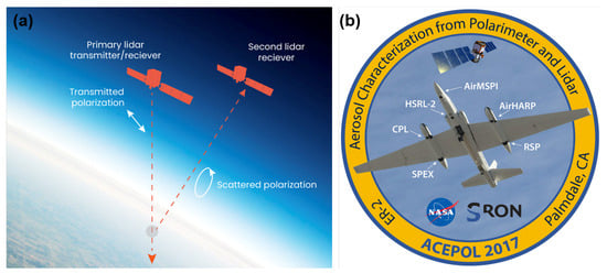
Figure 5. (a) P-lidar system with two satellites. (b) The ACEPOL field campaign emblem.
Airborne lidar provides mobility and a high signal-to-noise ratio (SNR), serving as a valuable complement to spaceborne lidar. In 2003, Dulac et al. utilized the airborne P-lidar known as ALEX to study multi-layer aerosol structures in the Eastern Mediterranean [90][146]. In 2012, Bo et al. developed an all-weather atmospheric aerosol–water vapor lidar system for aircraft. This system simultaneously captures backscatter at 355 nm/532 nm wavelengths, 532 nm depolarization, and nitrogen and water vapor molecular Raman signals, facilitating long-term monitoring of aerosols and water vapor [91][147]. Another famous airborne system is the Aerosol Characterization from Polarimeter and Lidar (ACEPOL), which was conducted in the fall of 2017 by NASA. Figure 5b shows the ACEPOL emblem, which illustrates the locations of the remote sensing instruments on the aircraft, with two on the fuselage and two in each wing pod [92][145]. Additionally, there is a growing emphasis on developing portable P-lidar systems. For instance in 2021, Kong et al. introduced a portable P-lidar system using a focal-plane-splitting scheme. This system is designed in a T-shaped structure, featuring a sealed transmitter and a detachable large-aperture receiver. It is well-suited for cost-effective, low-maintenance outdoor unmanned measurements [13].
As detection instruments continue to progress, research algorithms are also undergoing gradual evolution. Many solutions to the lidar equation for elastic scattering (e.g., Fernald et al. [93][148], Klett [94][149], Davis [95][150], Sasano and Nakane [96][151], and Collis and Russell [97][152]) have been proposed. Among these solutions, the Fernald analysis method treats atmospheric molecules and aerosol particles separately, making it the current pinnacle of inversion methods under development [98][153]. Building upon Fernald’s forward inversion technique, CALIOP employs the hybrid extinction retrieval algorithm (HERA), known for its flexibility and robustness as an iterative inversion method [99]. It utilizes hierarchical position data from the selective iterative boundary locator (SIBYL) and layer classification results from the scene classification algorithms (SCAs) to determine particle backscatter and extinction coefficients. It should be noted that Raman and HSRL, as the two typical systems to provide high-quality backscatter and extinction coefficients, have the potential for providing vertically resolved information about aerosol size/concentration [100][101][154,155]. For example, Thorsen et al. developed a comprehensive set of algorithms for processing the Raman lidar data to obtain the retrievals of aerosol extinction and feature detection. The details of the Raman algorithms for aerosol backscattering and extinction can be found in [102][103][156,157]. The HSRL data were processed in a manner akin to that of the Raman lidar data, ensuring alignment in terms of timestamps, altitudes, as well as temporal and vertical resolutions. While it is worth noting that the HSRL does not employ distinct low- and high-sensitivity channels, the processing and averaging approach for HSRL data is to mimic the processing of the Raman lidar low- and high-sensitivity channels for consistency. In 2017, based on the above algorithms, Ferrare et al. processed both the Raman lidar and HSRL to obtain a consistent set of profiles, with equivalent resolutions and averaging, across all wavelengths [104][158]. Recently, there have also been many researchers focused on developing advanced algorithms. For example, in 2022, the researchers in Italy employed a Bayesian parameter approach to infer the atmospheric particle size distribution [105][159]. In April of the same year, based on the spaceborne Aerosol and Cloud High-Spectral-Resolution Lidar (ACHSRL), capable of highly precise global aerosol and cloud detection, launched by China, Ju et al. proposed a retrieval algorithm for deriving aerosol and cloud optical properties from ACHSRL data, comparing it against end-to-end Monte Carlo simulations for validation. These efforts involved the use of the airborne prototype of ACHSRL [106][160].
2.2. Remote Sensing of Earth’s Surface
In applications related to terrain characterization, vegetation remote sensing, and other surface environmental studies, microwave radar has been proven to possess certain advantages. However, due to its relatively long wavelengths, it cannot provide high-resolution information about targets. lidar, on the other hand, operates at shorter wavelengths, enabling sufficient resolution of surface environmental structures and, thus, enhancing the performance of relevant applications.
In vegetation remote sensing, traditional lidars are mainly used for measuring height and echo intensity, thus inferring the three-dimensional surface structure of vegetation. One example is the Scanning lidar Imager of Canopies by Echo Recovery (SLICER) scanning lidar system [107][161]. SLICER used a 1064 nm neodymium-doped yttrium aluminum garnet (Nd:YAG) laser with a beam divergence angle of approximately 2 mrad. Under normal operating conditions, SLICER had a footprint diameter of about 9 m, and it could obtain the canopy height, above-ground biomass, cross-sectional area, and other forest characteristics. Another example is the vegetation canopy lidar, a spaceborne lidar system with three 1064 nm Nd:YAG lasers, providing a 25 m field of view at an altitude of 400 km. It can characterize the three-dimensional structure of the Earth’s surface on a global scale and offer improved global forest canopy height detection and biomass estimation [108][162]. However, all these lidars are non-polarimetric, and the ability to study the polarimetric properties of vegetation is of great significance.
In 1993, the NASA Goddard Space Flight Center made the first airborne laser polarization sensor (ALPS), i.e., a P-lidar, for the remote sensing of the Earth’s surface (vegetation) [41]. ALPS has a linearly polarized Nd:YAG laser source at both 1064 and 532 nm, with a detector field of view of approximately 0.03 rad. It can measure desired parameters such as the total backscatter and the polarization state. Using the ALPS system, researchers were able to distinguish unique cross-polarization signatures for different tree species, such as broadleaf and coniferous trees [41]. This system also revealed a significant correlation between near-infrared depolarization and crop parameters, specifically nitrogen fertilization. The depolarization spectral difference index proved to be effective for estimating crop yields [109][163]. However, one limitation of the ALPS system was its inability to capture the lidar return waveform, which prevented obtaining detailed information about the vertical structure of the vegetation canopy. To handle this issue, the University of Nebraska has refurbished the ALPS system and developed it into a multi-wavelength airborne P-lidar system, named MAPL [110][164]. MAPL’s receiver has four channels (dual-wavelength and dual-polarization detection) and records the entire lidar waveform. Therefore, it can study both vegetation canopy structure and the characterization of vegetation cross-polarization [111][165]. The same team also used MAPL to study the polarimetric reflectance from different tree species in the forest and proved its ability to detect different trees by analyzing the lidar waveform shapes, the depolarization ratios, and the reflectance percentages [112][166]. In 2018, Tian et al. proposed the measurement of co-polarized and cross-polarized components of maize leaves at a 532 nm laser wavelength [113][167]. They analyzed the depolarization differences under varying biochar contents and demonstrated that the laser depolarization ratio could serve as an indicator to monitor plant growth conditions.
P-lidars can also be applied for forest fire/smoke detection. By detecting and analyzing the backscattering process caused by the interaction between atmospheric particles and lasers, lidar can achieve precise measurements of smoke. However, traditional intensity-based lidar needs to find a commanding height for scanning, which is often hard to fulfill [114][115][168,169]. Moreover, due to the complexity of forest terrains, as they contain leaves and other obstacles, the lidar signals must pass through these leaves and obstacles, which makes it difficult to distinguish forest-fire smoke with a single-channel lidar. To solve this problem, Xian et al., in 2020, proposed a scanning P-lidar system to detect smoke from forest fires [116][108]. This system uses a 1064 nm pulsed laser and differentiates smoke from lidar signals contaminated by forest obstacles through the depolarization ratio.
A very important function of scanning or imaging lidar is its ability of 3D imaging in Urban remote sensing. The first polarization-modulated 3D lidar was proposed by Taboada and Tamburino in 1992 [117][170]. In order to improve the image quality, Chen et al. proposed an electron-multiplying charge-coupled-devices (EMCCDs)-based lidar system, in which the echo signal is separated into two orthogonal polarized components via a PBS. Such a polarization-modulated method improves the range accuracy of the objects of interest from 4.4 to 0.26 m with a gate opening range of 200 m [118][171]. In 2018, the same team found that the 3D imaging P-lidar had very promising performance in an FOV of 0.9 mrad [119][172]. The mentioned types of P-lidar, to some extent, belong to dual-channel P-lidar because they can only simultaneously acquire orthogonal polarization states. However, these systems require two cameras and a PBS to obtain orthogonal polarization states, making pixel-level alignment challenging [120][173]. In 2016, Jo et al. proposed a 3D flash P-lidar based on a micro-polarizer camera, as shown in Figure 6a, which can obtain the linear Stokes vector with a single shot [121][174], and achieved a spatial resolution and range precision of 0.12 mrad and 5.2 mm at 16 m, respectively [122][175].
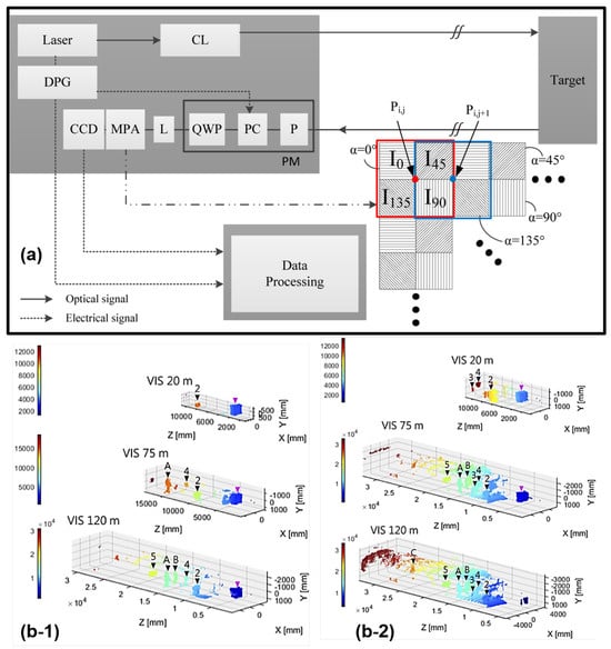
Figure 6. (a) P-lidar based on a polarization camera. (b) Reconstructed point clouds for (b-1) co-polarization and (b-2) cross-polarization configurations at 20 m, 75 m, and 120 m of visibility.
Another important application is autonomous driving, as lidar sensors are one of the key supporting technologies for implementing autonomous driving. Nunes-Pereira et al. demonstrated through experiments that the reflection signals from metallic car paints have distinct polarization characteristics [123][176]. Therefore, by using a P-lidar, distance measurements can be supplemented, thereby aiding in target classification. In their experiments, they utilized a custom-built P-lidar system, which employed a pulsed, linearly polarized 785 nm laser, a pair of 2D scanning galvanometer mirrors, and a linear polarizer positioned in front of the collection objective. The polarizer was alternately set for co-linear and cross-linear polarized detection. Including polarization into the lidar can improve autonomous driving performance in a dense atmosphere. In 2021, Ronen et al. introduced a model that combines traditional lidar and Stokes–Mueller formulations and conducted experiments inside an aerosol chamber [124][177]. The results showed that the use of a polarized source together with a cross-polarized receiver can improve the target-signal-to-atmospheric-signal ratio in a dense aerosol medium for a lidar system. Therefore, implementing polarimetric imaging techniques in lidars can enhance the performance of autonomous vehicles in poor-visibility conditions. Actually, this characteristic of polarization information can be found in many applications of polarization imaging [5][6][5,6]. In 2022, Ballesta-Garcia et al. studied the performance of P-lidar in a macro-scale fog chamber under controlled fog conditions and demonstrated many interesting findings [7]. For example, a system based on circularly polarized incident light and cross-polarized configuration helps to reduce the SNR, and a cross-polarized configuration enables the detection of objects while allowing the filtering out of most of the fog response, as shown in Figure 6b.
2.3. Ocean Remote Sensing
Aerosol observations utilize various passive and active remote sensing techniques, which can be applied to the ocean to better characterize hydrosols and enhance the atmospheric-correction process. While spectral radiance provides sensitivity to the absorption and scattering properties of constituents within the water column, polarized light emerging from the Earth system carries a wealth of information about the atmosphere, ocean, and surface, which remains underutilized in ocean color remote sensing. Polarized light originating beneath the ocean surface contains valuable microphysical details about hydrosols, including their shape, composition, and attenuation. Retrieving such information is challenging, if not impossible, using traditional scalar remote sensing methods alone. Moreover, polarimetric measurements offer opportunities to enhance the characterization and removal of atmospheric and surface reflectance that can interfere with ocean color measurements.
Kattawar et al. [125][178] were pioneers in conducting vector radiative transfer simulations for a coupled atmosphere–ocean system. It was not until 30 years later, in 2006, that Chowdhary et al. [126][179] first introduced models specifically addressing the polarized contribution from the ocean for photopolarimetric remote sensing observations of aerosols above the ocean [127][180]. This marked the beginning of increased interest in ocean-related applications of polarimetry. In 2007, Chami demonstrated the potential advantages of utilizing polarimetry to understand the optical and microphysical properties of suspended oceanic particles (hydrosols) through radiative transfer (RT) simulations [128][181]. In aquatic environments characterized by the prevalence of phytoplankton, the polarized reflectance at the top of the atmosphere exhibits a high degree of insensitivity to fluctuations in chlorophyll concentration. In 2009, Tonizzo et al. [129][182] developed a hyperspectral, multiangular polarimeter designed to measure the polarized light field in the ocean, accompanied by an RT closure analysis, which validated the theoretical analysis. Additionally, in 2010, Voss and Souaidia successfully measured the upwelling hemispheric polarized radiance at various visible wavelengths, revealing the geometrical dependence of polarized light [130][183].
Oceanic lidars can penetrate seawater to acquire highly accurate vertical profiles of multiple parameters within the ocean. Since the introduction of the first bathymetry lidar in 1968, various types of ocean lidars have been developed to assess different oceanic parameters and constituents. In particular, P-lidar, widely employed in oceanic studies, offers significant advantages in providing multiple oceanic parameters. Analyzing the elastic Mie backscattering signal, seawater’s optical properties can be estimated by retrieving the lidar attenuation coefficient within the laser’s penetration depth. Additionally, it can identify oceanic communities through the linear depolarization ratio, owing to the depolarization effect of non-spherical particles on incident light. In other words, oceanic P-lidar has achieved successful applications in various domains such as the retrieval of depolarization optical products in the upper ocean [52][67], the detection of phytoplankton layers [131][132][184,185], turbulence measurement [133][134][186,187], and marine biological population detection [135][136][188,189].
Over the past decade, oceanic P-lidar has found numerous applications in oceanographic research. For example, Vasilkov et al. employed an airborne P-lidar to generate profiles of the scattering coefficient and identified subsurface layers with high scattering properties during their field experiments [60][75]. Furthermore, Churnside et al. developed a radiative transfer equation for airborne polarized lidar returns, facilitating the detection of scattering layers, fish schools, seawater optical properties, and internal waves [52][67]. To expand the scope of ocean observing efforts, Collister et al. designed a shipborne lidar to investigate the combined impacts of particle composition and seawater multiple scattering based on the lidar’s linear depolarization ratio [137][190]. Behrenfeld et al. quantified phytoplankton biomass and diel vertical migration using the particulate backscattering coefficient and diffuse attenuation coefficient derived from the spaceborne P-lidar CALIOP [49][64]. Chen et al. observed the vertical distribution of subsurface phytoplankton layers in the South China Sea using a dual-wavelength airborne P-lidar [55][70]. Furthermore, Chen et al. introduced the planned “Guanlan” ocean remote sensing mission, featuring a near-nadir-pointing oceanic lidar and a dual-frequency interferometric altimetry system [55][70]. The oceanic lidar payload is expected to contribute significantly to theour understanding of the marine food chain and ecosystem by providing data with a 10 m vertical resolution within the euphotic layer, advancing our knowledge of both the dynamic and bio-optical characteristics of the oceanic mixed layer.
Marine biological population detection is also a promising application for oceanic lidars. Likely, the initial development of the theory for using lidar to detect fish schools was pioneered by Murphree et al. [138][191]. The first experimental trials, conducted in a controlled environment, were carried out by Swedish scientists [139][192]. In 1999, Churnside from the National Oceanic and Atmospheric Administration (NOAA) developed an airborne lidar for marine fisheries. This lidar is indeed a single-channel P-lidar and uses a polarizer in front of the telescope system to select either the component of the return that is co-polarized with the laser or the cross-polarized component [140][42]. Their results showed that one can see fish from an airborne P-lidar. In clear water, one can see to depths of 40–50 m, and in turbid waters, this depth penetration is reduced. In 2010, Churnside took a case study in Chesapeake Bay, by using the cross-polarized component as its contrast between fish, and the background-scattering level was greater than that of the co-polarized return. They found that the average depth penetration of lidar was 12 m, and the average depth of detected schools was 3 m [141][46]. In 2018, Shamanaev proposed a method of P-lidar sensing of marine fish schools based on a comparison of the numerical values of the lidar return power and depolarization with their threshold levels determined by the sea water extinction index in the fishery region [142][193].
Another example is jellyfish detection, which facilitates the acquisition of data encompassing jellyfish taxonomy, population metrics, spatial dispersion, and related particulars. This process holds a pivotal role within the ambit of jellyfish prevention and management. The existing methodologies for jellyfish detection presently exhibit limitations in terms of detection efficiency, precision, and vertical distribution insights. P-lidar holds the potential to accomplish remote sensing of individual jellyfish organisms. This advanced technology offers an efficient, cost-effective, and accurate means of monitoring variations in jellyfish distribution and population dynamics. Currently, there is a relatively limited amount of research focused on utilizing marine lidar for jellyfish detection. In 2015, Churnside et al. [136][189] employed an airborne polarized marine lidar to observe the phenomenon of hollow aggregations within jellyfish populations. Their findings were corroborated by sonar detection results, thereby substantiating the viability of using polarized marine lidar for jellyfish population detection. In August 2017, a shipborne polarimetric marine lidar, independently developed by the research team at Zhejiang University, China, conducted experimental measurements in the Yellow Sea [143][194]. During these experiments, it observed a wealth of strong scattering signals. By combining these data with video monitoring information, the team was able to identify the source of these signals as jellyfish, demonstrating that jellyfish in the same area exhibited clustering patterns in their optical characteristics. Furthermore, jellyfish signals from different regions had similar contrast, but varied depolarization rates, suggesting that the optical properties of jellyfish are closely related to their local environmental conditions.