Your browser does not fully support modern features. Please upgrade for a smoother experience.
Please note this is a comparison between Version 2 by Sirius Huang and Version 3 by Sirius Huang.
Scene classification in remote sensing images aims to categorize image scenes automatically into relevant classes like residential areas, cultivation land, forests, etc. The implementation of deep learning (DL) for scene classification is an emerging tendency, with an effort to achieve maximum accuracy.
- remote sensing
- deep learning
- scene classification
- convolutional neural networks
1. Introduction
The advancement in Earth observation technology has led to the availability of very high-resolution (VHR) images of the Earth’s surface. With the development of VHR images, it is possible to accurately identify and classify land use and land cover (LULC) [1], and the demands for such tasks are high. Scene classification in remote sensing images aims to categorize image scenes automatically into relevant classes like residential areas, cultivation land, forests, etc. [2], drawing considerable attention. In recent years, the application of scene classification in VHR satellite images is evident in disaster detection [3], land use [4][5][6][7][8][9], and urban planning [10]. The implementation of deep learning (DL) for scene classification is an emerging tendency in a current scenario, with an effort to achieve maximum accuracy.
In the early days of remote sensing, the spatial resolution of images was relatively low, resulting in the pixel size equivalent to the object of interest [11]. As a consequence, the studies on remote sensing classification were based on pixel-level [11][12][13]. Subsequently, the increment in spatial resolution reoriented the research to remote sensing classification on the object-level, which produced more enhanced classification than per-pixel analysis [14]. This approach dominated the remote sensing classification domain for decades, including [15][16][17][18][19][20]. However, the perpetual growth of remote sensing images facilitates capturing distinct object classes, rendering traditional pixel-level and object-level methods inadequate for accurate image classification. In such a scenario, scene-level classification became crucial to interpret the global contents of remote sensing images [21]. Thus, numerous experiments can be observed in scene-label analysis over the past few years [22][23][24][25][26]. Figure 1 illustrates the progression of classification approaches from pixel-level to object-level and finally to scene-level.
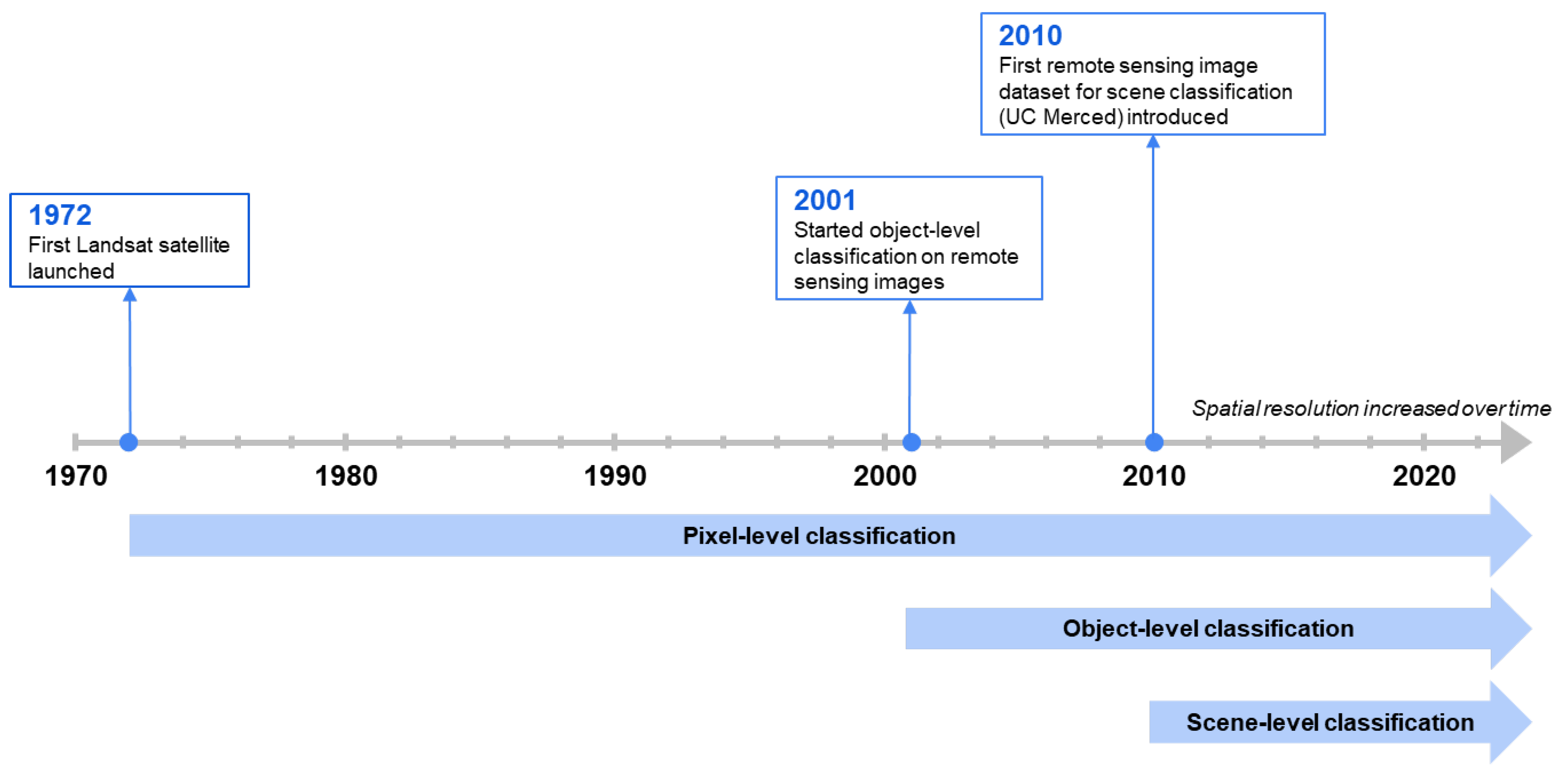
Figure 1. Timeline of remote sensing classification approaches. The spatial resolution of images increased over time, resulting in three classification levels: pixel-level, object-level, and scene-level classification.
The preliminary methods for remote sensing scene classification were predominantly relying on low-level features such as texture, color, gradient, and shape. Hand-crafted features like Scale-Invariant Feature Transform (SIFT), Gabor filters, local binary pattern (LBP), color histogram (CH), gray level co-occurrence matrix (GLCM), and histogram of oriented gradients (HOG) were designed to capture specific patterns or information from the low-level features [7][27][28][29][30]. These features are crafted by domain experts and are not learned automatically from data. The methods utilized on low-level features only rely on uniform texture and can not perform on complex scenes. On the other hand, methods on mid-level features extract more complex patterns with clustering, grouping, or segmentation [31][32]. The idea is to acquire local attributes from small regions or patches within an image and encode these local attributes to retrieve the intricate and detailed pattern [33]. The bag-of-visual-words (BoVW) model is a widely used mid-level approach for scene classification in the remote sensing field [34][35][36]. However, the limited representation capability of mid-level approaches has hindered breakthroughs in remote sensing image scene classification.
In recent times, DL models emerged as a solution to address the aforementioned limitations in low-level and mid-level methods. DL architectures implement a range of techniques, including Convolutional Neural Networks (CNNs) [37][38], Vision Transformers (ViT), and Generative Adversarial Networks (GANs), to learn discriminative features for effective feature extraction. For scene classification, the available datasets are grouped into diverse scenes. The DL architectures are either trained on these datasets to obtain the predicted scene class [39], or pretrained DL models are used to obtain derived classes from the same scene classes [40][41], depending upon the application. In the context of remote sensing scene classification, the experiments are mainly focused on achieving optimal scene prediction by implementing DL architectures. CNN architectures like Residual Network (ResNet) [42], AlexNet [43], GoogleNet [44], etc., are commonly used for remote sensing scene classification. Operations like fine-tuning [45], adding low-level and mid-level feature descriptors like LBP [46], BovW [47], etc., and developing novel architectures [33][48] are performed to obtain nearly ideal scene classification results. Furthermore, ViTs and GANs are also used to advance research and applications in this field.
2. High-Resolution Scene Classification Datasets
Multiple VHR remote sensing datasets are available for scene classification. The UC Merced Land Use Dataset (UC-Merced or UCM) [49] is a popular dataset obtained from the United States Geological Survey (USGS) National Map Urban Area Imagery collection covering US regions. Some of the classes belonging to this dataset are airplanes, buildings, forests, rivers, agriculture, beach, etc., depicted in Figure 2. The Aerial Image Dataset (AID) [23] is another dataset acquired from Google Earth Imagery with a higher number of images and classes than the UCM dataset. Table 1 lists some widely used datasets for scene recognition in the remote sensing domain. Some of the scene classes are common in multiple datasets. For instance, the “forest” class is included in UCM, WHU-RS19 [50], RSSCN7 [51], and NWPU-RESISC45 [52] datasets. However, there are variations in scene classes among different datasets. In addition, the number of images and their size and resolution of scene datasets varies in respective datasets. Thus, the selection of the dataset depends on the research objectives. Cheng et al. [52] proposed a novel large-scale dataset NWPU-RESISC45 with rich image variations and high within-class diversity and between-class similarity, addressing the problem of small-scale datasets, lack of variations, and diversity. Miao et al. [53] merged UCM, NWPU-RESISC45, and AID datasets to prepare a larger remote-sensing scene dataset for semi-supervised scene classification and attained a similar performance to the state-of-the-art methods. In these VHR datasets, multiple DL architectures have been conducted to obtain optimal accuracy.
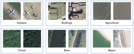
Figure 2. Sample images of some classes from the UCM dataset. In total, there are 21 classes in this dataset.
Table 1. Scene databases used for scene classification.
| Dataset | Number of Images | Classes | Image Size | Resolution (m) |
|---|---|---|---|---|
| UCM [49] | 2100 | 21 | 256 × 256 | 0.3 |
| AID [23] | 10,000 | 30 | 600 × 600 | 0.5–8 |
| WHU-RS19 [50] | 1005 | 19 | 600 × 600 | Up to 0.5 |
| NWPU-RESISC45 [52] | 31,500 | 45 | 256 × 256 | 0.2–30 |
| PatternNet [54] | 30,400 | 38 | 256 × 256 | 0.062–4.693 |
| OPTIMAL-31 [55] | 1860 | 31 | 256 × 256 | 0.3 |
| SIRI-WHU [56] | 2400 | 12 | 200 × 200 | 2 |
| RSSCN7 [51] | 2800 | 7 | 400 × 400 | - |
| RSI-CB256 [57] | >36,000 | 35 | 256 × 256 | 0.3–3 |
| RSI-CB128 [57] | >24,000 | 45 | 128 × 128 | 0.3–3 |
| KSA [58] | 3250 | 13 | 256 × 256 | 0.5–1 |
3. CNN-Based Scene Classification Methods
CNNs [59] effectively extract meaningful features from images by utilizing convolutional kernels and hierarchical layers. A typical CNN architecture includes a convolutional layer, pooling layer, Rectified Linear Unit (ReLU) activation layer, and fully connected (FC) layer [60] as shown in Figure 3. The mathematical formula for the output of each filter in a 2D convolutional layer is provided in Equation (1).
where 𝑓(·) represents the activation function, 𝑤𝑙𝑚,𝑛 is the weight associated with the connection between input feature map m and output feature map n, and 𝑏𝑙𝑚 denotes the bias term associated with output feature map n. The convolution layers learn features from input images, followed by the pooling layer, which reduces computational complexity while retaining multi-scale information. The ReLU activation function introduces non-linearity to the network, allowing for the modeling of complex relationships and enhancing the network’s ability to learn discriminative features. The successive use of convolutional and pooling layers allows the network to learn increasingly complex and abstract features at different scales. The first few initial layers capture low-level features such as edges and textures, while deeper layers learn high-level features and global structures [61]. The FC layers serve as a means of mapping the learned features to the final output space, enabling the network to make predictions based on the extracted information. In a basic CNN structure, the output of an FC layer is fed into either a softmax or a sigmoid activation function for classification tasks. However, the majority of parameters are occupied by an FC layer, increasing the possibility of overfitting. Dropout is implemented to counter this problem [62]. To minimize loss and improve the model’s performance, several optimizers like Adam [63] and stochastic gradient descent (SGD) [64] are prevalent in research.
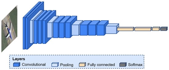
Figure 3. A typical CNN architecture. Downsampling operations such as pooling and convolution layers allow the capture of multi-scale information from the input image, finally classifying them with an FC layer.
Multiple approaches have been explored to optimize the feature extraction process for accurate remote sensing scene classification using CNNs. They are sub-divided into two categories: pretrained CNNs and CNNs trained from scratch.
3.1. Pretrained CNNs for Feature Extraction
Collecting and annotating data for larger remote sensing scene datasets increases costs and is a laborious task. To address the scarcity of data in the remote sensing domain, researchers often utilize terrestrial image datasets such as ImageNet [65] and PlacesCNN [66], which contain a large number of diverse images from various categories. Wang et al. [67] described the local similarity between remote sensing scene image and natural image scenes. By leveraging pretrained models trained on these datasets, the CNN algorithms can benefit from the learned features and generalize well to remote sensing tasks with limited labeled data. This process is illustrated in Figure 4, showcasing the role of pretrained CNNs.
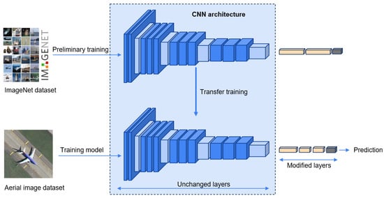
Figure 4. Pretrained CNN utilized for feature extraction from the aerial image dataset. The weight parameters of CNN pretrained on the ImageNet dataset are transferred to the new CNN. Top layers are replaced with a custom layer configuration fitting to the target concept.
In 2015, Penatti et al. [30] introduced pretrained CNN on ImageNet into remote sensing scene classification, discovering better classification results for the UCM dataset than low-level descriptors. In a diverse large-scale dataset named NWPU-RESISC45, three popular pretrained CNNs: AlexNet [62], VGG-16 [68] and GoogLeNet [69], improved the performance by 30% minimum compared to handcrafted and unsupervised feature learning methods [52]. NWPU-RESISC45 dataset is ambiguous due to high intra-class diversity and inter-class similarity. Sen et al. [70] adopted a hierarchical approach to mitigate the misclassification. Their method is divided into two levels: (i) all 45 classes are rearranged into 5 main classes (Transportation, Water Areas, Buildings, Constructed Lands, Natural Lands), and (ii) the 45 sub-levels are trained in each class. DenseNet-121 [71] pretrained on ImageNet is used as a feature extractor in both levels. Al et al. [72] combined four scene datasets, namely UCM, AID, NPWU, and PatternNet, to construct a heterogeneous scene dataset. For suitability, the 12 shared classes are filtered to utilize an MB-Net architecture, which is based on pretrained ResNet-50 [73]. MB-Net is designed to capture collective knowledge from three labeled source datasets and perform scene classification on a remaining unlabeled target dataset. Shawky et al. [74] brought a data augmentation strategy for CNN-MLP architecture with Xception [75] as a feature extractor. Sun et al. [76] obtained multi-scale ground objects using multi-level convolutional pyramid semantic fusion (MCPSF) architecture and differentiated intricate scenes consisting of diverse ground objects.
Yu et al. [77] introduced a feature fusion strategy in which CNNs are utilized to extract features from both the original image and a processed image obtained through saliency detection. The extracted features from these two sources are then fused together to produce more discriminative features. Ye et al. [78] proposed parallel multi-stage (PMS) architecture based on the GoogleNet backbone to learn features individually from three hierarchical levels: low-, middle-, and high-level, prior to fusion. Dong et al. [79] integrated a Deep Convolutional Neural Network (DCNN) with Broad Learning System (BLS) [80] for the first time in the remote sensing scene classification domain to extract shallow features and named it FDPResNet. The DCNN implemented ResNet-101 pretrained on ImageNet as a backbone on both shallow and deep features and further fused and passed to the BLS system for classification. CNN architectures for remote sensing scene classification vary in design with the incorporation of additional techniques and methodologies. However, the widely employed approaches include LBP-based, fine-tuning, parameter reduction, and attention mechanism methods.
LBP-based pretrained CNNs: LBP is a widely used robust low-level descriptor for recognizing textures [81]. In 2018, Anwer et al. [46] proposed Tex-Net architecture, which combined an original RGB image with a texture-coded mapped LBP image. The late fusion strategy (Tex-Net-LF) performed better than early fusion (Tex-Net-EF). Later, Yu et al. [82], who previously introduced the two-stream deep fusion framework [77], adopted the same concept to integrate the LBP-coded image as a replacement for the processed image obtained through saliency detection. However, they conducted a combination of previously proposed and new experiments using the LBP-coded mapped image and fused the features together. Huang et al. [83] stated that two-stream architectures solely focus on RGB image stream and overlook texture-containing images. Therefore, CTFCNN architecture based on pretrained CaffeNet [84] extracted three kinds of features: (i) convolutional features from multiple layers, wherein each layer improved bag-of-visual words (iBoVW) method represented discriminating information, (ii) FC features, and (iii) LBP-based FC features. Compared to traditional BoVW [35], the iBoVW coding method achieved rational representation.
Fine-tuned pretrained CNNs: Cheng et al. [52] not only used pretrained CNNs for feature extraction from the NWPU-RESISC45 dataset, they further fine-tuned the increasing learning rate in the last layer to gain better classification results. For the same dataset, Yang et al. [85] fine-tuned parameters utilized on three CNN models: VGG-16 and DenseNet-161 pretrained on ImageNet used as deep-learning classifier training, and feature pyramid network (FPN) [86] pretrained on Microsoft Coco (Common Objects in Context) [87] for deep-learning detector training. The combination of DenseNet+FPN exhibited exceptional performance. Zhang et al. [33] used the hit and trial technique to set the hyperparameters to achieve better accuracy. Petrovska et al. [88] implemented linear learning rate decay, which decreases the learning rate over time, and cyclical learning rates [89]. The improved accuracy utilizing fine-tuning on pretrained CNNs validates the statement made by Castelluccio et al. [90] in 2015.
Parameters reduction: CNN architectures exhibit a substantial amount of parameters, such as VGG-16, which comprises approximately 138 million parameters [91]. The large number of parameters is one of the factors for over-fitting [92][93]. Zhang et al. [94] utilized DenseNet, which is known for its parameter efficiency, with around 7 million parameters. Yu et al. [95] integrated light-weighted CNN MobileNet-v2 [96] with feature fusion bilinear model [97] and termed the architecture as BiMobileNet. BiMobileNet featured a parameter count of 0.86 million, which is six, eleven, and eighty-five times lower than the parameter numbers reported in [82], [45] and [98], respectively, while achieving better accuracy.
Attention mechanism: In the process of extracting features from entire images, it is essential to consider that images contain various objects and features. Therefore, selectively focusing on critical parts and disregarding irrelevant ones becomes crucial. Zhao et al. [99] added a channel-spatial attention [100] module (CBAM) following each residual dense block (RDB) based on DenseNet-101 backbone pretrained on ImageNet. CBAM helps to learn meaningful features in both channel and spatial dimensions [101]. Ji et al. [102] proposed an attention network based on the VGG-VD16 network that localizes discriminative areas in three different scales. The multiscale images are fed to sub-network CNN architectures and further fused for classification. Zhang et al. [103] introduced a multiscale attention network (MSA-Network), where the backbone is ResNet. After each residual block, the multiscale module is integrated to extract multiscale features. The channel and position attention (CPA) module is added after the last multiscale module to extract discriminative regions. Shen et al. [104] incorporated two models, namely ResNet-50 and DenseNet-121, to fulfill the insufficiency of single CNN models. Both models captured low, middle, and high-level features and combined them with a grouping-attention-fusion strategy. Guo et al. [105] proposed a multi-view feature learning network (MVFL) divided into three branches: (i) channel-spatial attention to localize discriminative areas, (ii) triplet metric branch, and (iii) center metric branch to increase interclass distance and decrease intraclass distance. Zhao et al. [106] designed an enhanced attention module (EAM) to enhance the ability to understand more discriminative features. In EAM, two depthwise dilated convolution branches are utilized, each branch having different dilated rates. Dilated convolutions enhance the receptive fields without escalating the parameter count. They effectively capture multiscale contextual information and improve the network’s capacity to learn features. The two branches are merged with depthwise convolutions to decrease the dimensionality. Hu et al. [107] introduced a multilevel inheritance network (MINet), where FPN based on ResNet-50 is adopted to acquire multilayer features. Subsequently, an attention mechanism is employed to augment the expressive capacity of features at each level. For the fusion of features, the feature weights across different levels are computed by leveraging the SENet [108] approach.
3.2. CNNs Trained from Scratch
Pretrained CNNs are typically trained on large-scale datasets such as ImageNet, which are not adaptable to the specific characteristics of the target dataset. Modifying pretrained CNNs is inconvenient due to the complexity and compatibility of CNNs. Although pretrained CNNs attained outstanding classification results, Zhang et al. [109] addressed complexity in pretrained CNNs due to the extensive parameter size and implemented a light-weighted CNN MobileNet-v2 with dilated convolution and channel attention. He et al. [110] introduced a skip-connected covariance (SCCov) network, where a skip connection is added along with covariance pooling. The SCCov architecture reduced the parameter number with better scene classification. Zhang et al. [111] proposed a gradient-boosting random convolutional network to assemble various non-pretrained deep neural networks (DNNs). A simplified representation of CNN architectures trained from scratch is illustrated in Figure 3. This CNN is solely based on a dataset to be trained without the involvement of pretrained CNN on a specific dataset.
4. Vision Transformer-Based Scene Classification Methods
The ViT [112] model can perform image feature extraction without relying on convolutional layers. This model utilizes a transformer architecture [113], initially introduced for natural language processing. In ViT, an input image undergoes partitioning into fixed-size patches, and each patch is then transformed into a continuous vector through a process known as linear embedding. Moreover, position embeddings are added to the patch embeddings to retain positional information. Subsequently, a set of sequential patches (Equation (2)) are fed into the transformer encoder, which consists of alternating layers of Multi-head Self-Attention (MSA) [113] (Equation (3)) and multi-layer perceptron (MLP) (Equation (4)). Layernorm (LN) [114] is implemented prior to both MSA and MLP to reduce training time and stabilize the training process. Residual connections are applied after every layer to improve the performance. The MLP has two layers with a Gaussian Error Linear Unit (GELU) [115] activation function. In the final layer of the encoder, the first element of the sequence is passed to an external head classifier for prediction (Equation (5)). Figure 5 illustrates the ViT architecture for remote sensing scene classification.
where 𝑥class represents the embedding for the class token. 𝑥𝑖𝑝E denotes the embeddings of different patches flattened from the original images, concatenated with 𝑥class. ℝ(𝑃2·𝐶)×𝐷 is a matrix representing patch embeddings where P is patch size, C is the number of channels, and D is the embedding dimension. Positional embedding 𝐸𝑝𝑜𝑠 is added to patches, accounting for 𝑁+1 positions (including class token), each in a D-dimensional space.
where 𝑧′𝑙 is the output of the MSA layer, applied after LN to the (𝑙−1)-th layer’s output 𝑧𝑙−1 (i.e., 𝑧0), incorporating a residual connection. L represents the total number of layers in the transformer.
where 𝑧𝑙 is the output of the MLP layer, applied after LN to the 𝑧′𝑙 from the (𝑙−1)-th layer, incorporating a residual connection. L represents the total number of layers in the transformer.
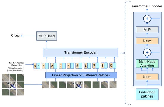
Figure 5. A ViT architecture. A remote sensing scene image is partitioned into fixed-size patches, each of them linearly embedded, and positional embeddings are added. The resulting sequence of vectors are fed to a transformer encoder for classification.
ViT performs exceptionally well in capturing contextual features. Bazi et al. [116] introduced ViT for remote sensing scene classification and obtained a promising result compared to state-of-the-art CNN-based scene classification methods. Their method involves data augmentation strategies to improve classification accuracy. Furthermore, the network is compressed by pruning to reduce the model size. Bashmal et al. [117] utilized a data-efficient image transformer (DeiT), which is trained by knowledge distillation with a smaller dataset and showed potential results. Bi et al. [118] used the combination of ViT and supervised contrastive learning (CL) [119], named ViT-CL, to increase the robustness of the model by learning more discriminative features. ViT performs exceptionally well in capturing contextual features. However, they face limitations in learning local information. Moreover, their computational complexity is significantly high [120]. Peng et al. [121] addressed the challenge and introduced a local–global interactive ViT (LG-ViT). In LG-ViT architecture, images are partitioned to learn features in two different scales: small and large. ViT blocks learn from both scales to handle the problem of scale variation. In addition, a global-view network is implemented to learn global features from a whole image. The features obtained from the global-view network are embedded with local representation branches, which enhance local–global feature interaction.
CNNs excel at preserving local information but lack the ability to comprehensively capture global contextual features. ViTs are well-suited to learn long-range contextual relations. The hybrid approach of using CNNs and transformers leverages the strengths of both architectures to improve classification performance. Xu et al. [120] integrated ViT and CNN to harness the strength of CNN. In their study, ViT is used to extract rich contextual information, which is transferred to the ResNet-18 architecture. Tang et al. [122] proposed an efficient multiscale transformer and cross-level attention learning (EMTCAL), which also combines CNN with a transformer to extract maximum information. They employed ResNet-34 as a feature extractor in the CNN model. Zhang et al. [123] proposed a remote sensing transformer (TRS) to capture the global context of the image. TRS combines self-attention with ResNet through the Multi-Head Self-Attention layer (MHSA), replacing the conventional 3 × 3 spatial convolutions in the bottleneck. Additionally, the approach incorporates multiple pure transformer encoders, leveraging attention mechanisms to enhance the learning of representations. Wang et al. [124] utilized pretrained Swin Transformer [125] to capture features at multilayer followed by patch merging to concatenate the patches (except in the last block), with these two elements forming the Swin Transformer Block (STB). The multilevel features obtained from STB are eventually merged with the inspired technique [86], then further compressed using convolutions within the adaptive feature compression module because of redundancy in multiple features. Guo et al. [126] integrated Channel-Spatial Attention (CSA) into the ViT [112] and termed the architecture Channel-Spatial Attention Transformers (CSAT). The combined CSAT model accurately acquires and preserves both local and global knowledge.
5. GAN-Based Scene Classification Methods
Supervised learning methods effectively perform remote sensing scene classification. However, due to limited labeled scene images, Miao et al. merged UCM, NWPU-RESISC45, and AID datasets to create larger remote-sensing scene datasets [53]. Annotating samples manually for labeling scenes is laborious and expensive. GAN [127] can extract meaningful information using unlabeled data. GAN is centered around two models: the generator and the discriminator, illustrated in Figure 6. The generator is trained to create synthetic data that resemble real data, aiming to deceive the discriminator. On the other hand, the discriminator is trained to distinguish between the generated (fake) data and the real data [128]. The overall objective of GAN is to achieve a competitive interplay between these two models, driving the generator to produce increasingly realistic data samples while the discriminator becomes better at detecting the generated data. In Equation (6), the value function describes the training process of GAN as a minimax game.
where the input from the latent space z is provided to the generator G to generate synthetic image G(z). G(z) is further fed to the discriminator D, alongside the real image x. The discriminator predicts both samples as synthetic (0) or real (1) based on its judgment. This process optimizes G and D through a dynamic interplay. G trains to minimize log(1−𝐷(𝐺(𝑧))), driving it to create synthetic images that resemble real ones. Simultaneously, D trains to maximize log(𝐷(𝑥)) + log(1−𝐷(𝐺(𝑧))), refining its ability to distinguish real from synthetic samples.
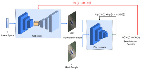
Figure 6. A GAN architecture consisting of generator G and discriminator D. G generates synthetic image G(z) from the latent space z. G(z) and real image x are then fed into the D, which is responsible for distinguishing between G(z) and x.
Lin et al. [129] acknowledged the unavailability of sufficient labeled data for remote sensing scene classification, which led them to introduce multiple-layer feature-matching generative adversarial networks (MARTA GANs). MARTA GANs fused mid-level features with global features for learning better representations by a descriptor. Xu et al. [130] replaced ReLU with scaled exponential linear units (SELU) [131] activation, enhancing GAN’s ability to produce high-quality images. Ma et al. [132] addressed that samples generated by GAN are solely used for self-training and introduced a new approach, SiftingGAN, to generate a significant number of authentic labeled samples. Wei et al. [133] introduced multilayer feature fusion Wasserstein GAN (MF-WGANs), where the multi-feature fusion layer is subsequent to the discriminator to learn mid-level and high-level feature information.
In unsupervised learning methods, labeled image scenes remain unexplored. However, leveraging annotations can significantly enhance classification capabilities. Therefore, Yan et al. [134] incorporated semi-supervised learning into GAN, aiming to exploit the benefits of labeled images and enhance classification performance. Miao et al. [53] introduced a semi-supervised representation consistency Siamese network (SS-RCSN), which incorporates Involution-GAN for unsupervised feature learning and a Siamese network to measure the similarity between labeled and unlabeled data in a high-dimensional space. Additionally, representation consistency loss in the Siamese network aids in minimizing the disparities between labeled and unlabeled data.
References
- Gómez-Chova, L.; Tuia, D.; Moser, G.; Camps-Valls, G. Multimodal classification of remote sensing images: A review and future directions. Proc. IEEE 2015, 103, 1560–1584.
- Li, Y.; Zhu, Z.; Yu, J.G.; Zhang, Y. Learning deep cross-modal embedding networks for zero-shot remote sensing image scene classification. IEEE Trans. Geosci. Remote Sens. 2021, 59, 10590–10603.
- Cheng, G.; Guo, L.; Zhao, T.; Han, J.; Li, H.; Fang, J. Automatic landslide detection from remote-sensing imagery using a scene classification method based on BoVW and pLSA. Int. J. Remote Sens. 2013, 34, 45–59.
- Othman, E.; Bazi, Y.; Alajlan, N.; Alhichri, H.; Melgani, F. Using convolutional features and a sparse autoencoder for land-use scene classification. Int. J. Remote Sens. 2016, 37, 2149–2167.
- Kunlun, Q.; Xiaochun, Z.; Baiyan, W.; Huayi, W. Sparse coding-based correlaton model for land-use scene classification in high-resolution remote-sensing images. J. Appl. Remote Sens. 2016, 10, 042005.
- Zhao, L.; Tang, P.; Huo, L. A 2-D wavelet decomposition-based bag-of-visual-words model for land-use scene classification. Int. J. Remote Sens. 2014, 35, 2296–2310.
- Chen, C.; Zhang, B.; Su, H.; Li, W.; Wang, L. Land-use scene classification using multi-scale completed local binary patterns. Signal, Image Video Process. 2016, 10, 745–752.
- Weng, Q.; Mao, Z.; Lin, J.; Liao, X. Land-use scene classification based on a CNN using a constrained extreme learning machine. Int. J. Remote Sens. 2018, 39, 6281–6299.
- Qi, K.; Wu, H.; Shen, C.; Gong, J. Land-use scene classification in high-resolution remote sensing images using improved correlatons. IEEE Geosci. Remote Sens. Lett. 2015, 12, 2403–2407.
- Xia, J.; Ding, Y.; Tan, L. Urban remote sensing scene recognition based on lightweight convolution neural network. IEEE Access 2021, 9, 26377–26387.
- Janssen, L.L.; Middelkoop, H. Knowledge-based crop classification of a Landsat Thematic Mapper image. Int. J. Remote Sens. 1992, 13, 2827–2837.
- Ji, M.; Jensen, J.R. Effectiveness of subpixel analysis in detecting and quantifying urban imperviousness from Landsat Thematic Mapper imagery. Geocarto Int. 1999, 14, 33–41.
- Tuia, D.; Ratle, F.; Pacifici, F.; Kanevski, M.F.; Emery, W.J. Active learning methods for remote sensing image classification. IEEE Trans. Geosci. Remote Sens. 2009, 47, 2218–2232.
- Blaschke, T.; Strobl, J. What’s wrong with pixels? Some recent developments interfacing remote sensing and GIS. Z. Geoinformationssyst. 2001, 4, 12–17.
- Blaschke, T. Object based image analysis for remote sensing. ISPRS J. Photogramm. Remote Sens. 2010, 65, 2–16.
- Blaschke, T.; Lang, S.; Hay, G. Object-Based Image Analysis: Spatial Concepts for Knowledge-Driven Remote Sensing Applications; Springer Science & Business Media: Berlin/Heidelberg, Germany, 2008.
- Hay, G.J.; Blaschke, T.; Marceau, D.J.; Bouchard, A. A comparison of three image-object methods for the multiscale analysis of landscape structure. ISPRS J. Photogramm. Remote Sens. 2003, 57, 327–345.
- Li, H.; Gu, H.; Han, Y.; Yang, J. Object-oriented classification of high-resolution remote sensing imagery based on an improved colour structure code and a support vector machine. Int. J. Remote Sens. 2010, 31, 1453–1470.
- Blaschke, T.; Hay, G.J.; Kelly, M.; Lang, S.; Hofmann, P.; Addink, E.; Feitosa, R.Q.; Van der Meer, F.; Van der Werff, H.; Van Coillie, F.; et al. Geographic object-based image analysis–towards a new paradigm. ISPRS J. Photogramm. Remote Sens. 2014, 87, 180–191.
- Blaschke, T.; Burnett, C.; Pekkarinen, A. Image segmentation methods for object-based analysis and classification. In Remote Sensing Image Analysis: Including the Spatial Domain; Springer: Berlin/Heidelberg, Germany, 2004; pp. 211–236.
- Cheng, G.; Xie, X.; Han, J.; Guo, L.; Xia, G.S. Remote sensing image scene classification meets deep learning: Challenges, methods, benchmarks, and opportunities. IEEE J. Sel. Top. Appl. Earth Obs. Remote Sens. 2020, 13, 3735–3756.
- Cheng, G.; Li, Z.; Yao, X.; Guo, L.; Wei, Z. Remote sensing image scene classification using bag of convolutional features. IEEE Geosci. Remote Sens. Lett. 2017, 14, 1735–1739.
- Xia, G.S.; Hu, J.; Hu, F.; Shi, B.; Bai, X.; Zhong, Y.; Zhang, L.; Lu, X. AID: A benchmark data set for performance evaluation of aerial scene classification. IEEE Trans. Geosci. Remote Sens. 2017, 55, 3965–3981.
- Zhong, Y.; Cui, M.; Zhu, Q.; Zhang, L. Scene classification based on multifeature probabilistic latent semantic analysis for high spatial resolution remote sensing images. J. Appl. Remote Sens. 2015, 9, 095064.
- Li, X.; Guo, Y. Multi-level adaptive active learning for scene classification. In Proceedings of the Computer Vision–ECCV 2014: 13th European Conference, Zurich, Switzerland, 6–12 September 2014; Part VII. pp. 234–249.
- Wang, X.; Duan, L.; Ning, C. Global context-based multilevel feature fusion networks for multilabel remote sensing image scene classification. IEEE J. Sel. Top. Appl. Earth Obs. Remote Sens. 2021, 14, 11179–11196.
- Yang, Y.; Newsam, S. Comparing SIFT descriptors and Gabor texture features for classification of remote sensed imagery. In Proceedings of the 2008 15th IEEE International Conference on Image Processing, San Diego, CA, USA, 12–15 October 2008; pp. 1852–1855.
- dos Santos, J.A.; Penatti, O.A.; Torres, R.d.S. Evaluating the potential of texture and color descriptors for remote sensing image retrieval and classification. In Proceedings of the International Conference on Computer Vision Theory and Applications, Angers, France, 17–21 May 2010; Volume 2, pp. 203–208.
- Luo, B.; Jiang, S.; Zhang, L. Indexing of remote sensing images with different resolutions by multiple features. IEEE J. Sel. Top. Appl. Earth Obs. Remote Sens. 2013, 6, 1899–1912.
- Penatti, O.A.; Nogueira, K.; Dos Santos, J.A. Do deep features generalize from everyday objects to remote sensing and aerial scenes domains? In Proceedings of the IEEE Conference on Computer Vision and Pattern Recognition Workshops, Boston, MA, USA, 7–12 June 2015; pp. 44–51.
- Yang, A.Y.; Wright, J.; Ma, Y.; Sastry, S.S. Unsupervised segmentation of natural images via lossy data compression. Comput. Vis. Image Underst. 2008, 110, 212–225.
- Carreira, J.; Sminchisescu, C. CPMC: Automatic object segmentation using constrained parametric min-cuts. IEEE Trans. Pattern Anal. Mach. Intell. 2011, 34, 1312–1328.
- Zhang, W.; Tang, P.; Zhao, L. Remote sensing image scene classification using CNN-CapsNet. Remote Sens. 2019, 11, 494.
- Zhou, L.; Zhou, Z.; Hu, D. Scene classification using a multi-resolution bag-of-features model. Pattern Recognit. 2013, 46, 424–433.
- Zhu, Q.; Zhong, Y.; Zhao, B.; Xia, G.S.; Zhang, L. Bag-of-visual-words scene classifier with local and global features for high spatial resolution remote sensing imagery. IEEE Geosci. Remote Sens. Lett. 2016, 13, 747–751.
- Zhao, L.J.; Tang, P.; Huo, L.Z. Land-use scene classification using a concentric circle-structured multiscale bag-of-visual-words model. IEEE J. Sel. Top. Appl. Earth Obs. Remote Sens. 2014, 7, 4620–4631.
- Jogin, M.; Madhulika, M.S.; Divya, G.D.; Meghana, R.K.; Apoorva, S. Feature extraction using convolution neural networks (CNN) and deep learning. In Proceedings of the 2018 3rd IEEE International Conference on Recent Trends in Electronics, Information & Communication Technology (RTEICT), Bangalore, India, 18–19 May 2018; pp. 2319–2323.
- Scarpa, G.; Gargiulo, M.; Mazza, A.; Gaetano, R. A CNN-based fusion method for feature extraction from sentinel data. Remote Sens. 2018, 10, 236.
- Zhou, B.; Lapedriza, A.; Khosla, A.; Oliva, A.; Torralba, A. Places: A 10 million image database for scene recognition. IEEE Trans. Pattern Anal. Mach. Intell. 2017, 40, 1452–1464.
- Thapa, A.; Neupane, B.; Horanont, T. Object vs Pixel-based Flood/Drought Detection in Paddy Fields using Deep Learning. In Proceedings of the 2022 12th International Congress on Advanced Applied Informatics (IIAI-AAI), Kanazawa, Japan, 2–7 July 2022; pp. 455–460.
- Thapa, A.; Horanont, T.; Neupane, B. Parcel-Level Flood and Drought Detection for Insurance Using Sentinel-2A, Sentinel-1 SAR GRD and Mobile Images. Remote Sens. 2022, 14, 6095.
- Wang, M.; Zhang, X.; Niu, X.; Wang, F.; Zhang, X. Scene classification of high-resolution remotely sensed image based on ResNet. J. Geovisualization Spat. Anal. 2019, 3, 16.
- Hu, F.; Xia, G.S.; Hu, J.; Zhang, L. Transferring deep convolutional neural networks for the scene classification of high-resolution remote sensing imagery. Remote Sens. 2015, 7, 14680–14707.
- Wang, Q.; Huang, W.; Xiong, Z.; Li, X. Looking closer at the scene: Multiscale representation learning for remote sensing image scene classification. IEEE Trans. Neural Netw. Learn. Syst. 2020, 33, 1414–1428.
- Xie, J.; He, N.; Fang, L.; Plaza, A. Scale-free convolutional neural network for remote sensing scene classification. IEEE Trans. Geosci. Remote Sens. 2019, 57, 6916–6928.
- Anwer, R.M.; Khan, F.S.; Van De Weijer, J.; Molinier, M.; Laaksonen, J. Binary patterns encoded convolutional neural networks for texture recognition and remote sensing scene classification. ISPRS J. Photogramm. Remote Sens. 2018, 138, 74–85.
- Zhao, W.; Du, S. Scene classification using multi-scale deeply described visual words. Int. J. Remote Sens. 2016, 37, 4119–4131.
- Sitaula, C.; KC, S.; Aryal, J. Enhanced Multi-level Features for Very High Resolution Remote Sensing Scene Classification. arXiv 2023, arXiv:2305.00679.
- Yang, Y.; Newsam, S. Bag-of-visual-words and spatial extensions for land-use classification. In Proceedings of the 18th SIGSPATIAL International Conference on Advances in Geographic Information Systems, San Jose, CA, USA, 2–5 November 2010; pp. 270–279.
- Xia, G.S.; Yang, W.; Delon, J.; Gousseau, Y.; Sun, H.; Maître, H. Structural High-resolution Satellite Image Indexing. In Proceedings of the ISPRS TC VII Symposium—100 Years ISPRS, Vienna, Austria, 5–7 July 2010; Volume XXXVIII, pp. 298–303.
- Zou, Q.; Ni, L.; Zhang, T.; Wang, Q. Deep learning based feature selection for remote sensing scene classification. IEEE Geosci. Remote Sens. Lett. 2015, 12, 2321–2325.
- Cheng, G.; Han, J.; Lu, X. Remote sensing image scene classification: Benchmark and state of the art. Proc. IEEE 2017, 105, 1865–1883.
- Miao, W.; Geng, J.; Jiang, W. Semi-supervised remote-sensing image scene classification using representation consistency siamese network. IEEE Trans. Geosci. Remote Sens. 2022, 60, 5616614.
- Zhou, W.; Newsam, S.; Li, C.; Shao, Z. PatternNet: A benchmark dataset for performance evaluation of remote sensing image retrieval. ISPRS J. Photogramm. Remote Sens. 2018, 145, 197–209.
- Wang, Q.; Liu, S.; Chanussot, J.; Li, X. Scene classification with recurrent attention of VHR remote sensing images. IEEE Trans. Geosci. Remote Sens. 2018, 57, 1155–1167.
- Zhao, B.; Zhong, Y.; Xia, G.S.; Zhang, L. Dirichlet-derived multiple topic scene classification model for high spatial resolution remote sensing imagery. IEEE Trans. Geosci. Remote Sens. 2015, 54, 2108–2123.
- Li, H.; Tao, C.; Wu, Z.; Chen, J.; Gong, J.; Deng, M. RSI-CB: A large scale remote sensing image classification benchmark via crowdsource data. arXiv 2017, arXiv:1705.10450.
- Othman, E.; Bazi, Y.; Melgani, F.; Alhichri, H.; Alajlan, N.; Zuair, M. Domain adaptation network for cross-scene classification. IEEE Trans. Geosci. Remote Sens. 2017, 55, 4441–4456.
- Liu, Y.H. Feature extraction and image recognition with convolutional neural networks. J. Phys. Conf. Ser. 2018, 1087, 062032.
- Coşkun, M.; Uçar, A.; Yildirim, Ö.; Demir, Y. Face recognition based on convolutional neural network. In Proceedings of the 2017 International Conference on Modern Electrical and Energy Systems (MEES), Kremenchuk, Ukraine, 15–17 November 2017; pp. 376–379.
- Guo, P.; Valanarasu, J.M.J.; Wang, P.; Zhou, J.; Jiang, S.; Patel, V.M. Over-and-under complete convolutional rnn for mri reconstruction. In Proceedings of the Medical Image Computing and Computer Assisted Intervention–MICCAI 2021: 24th International Conference, Strasbourg, France, 27 September–1 October 2021; Part VI. pp. 13–23.
- Krizhevsky, A.; Sutskever, I.; Hinton, G.E. Imagenet classification with deep convolutional neural networks. Commun. ACM 2017, 60, 84–90.
- Kingma, D.P.; Ba, J. Adam: A method for stochastic optimization. arXiv 2014, arXiv:1412.6980.
- Bottou, L. Large-scale machine learning with stochastic gradient descent. In Proceedings of the COMPSTAT’2010: 19th International Conference on Computational Statistics, Paris, France, 22–27 August 2010; pp. 177–186.
- Deng, J.; Dong, W.; Socher, R.; Li, L.J.; Li, K.; Fei-Fei, L. Imagenet: A large-scale hierarchical image database. In Proceedings of the 2009 IEEE Conference on Computer Vision and Pattern Recognition, Miami, FL, USA, 20–25 June 2009; pp. 248–255.
- Zhou, B.; Lapedriza, A.; Xiao, J.; Torralba, A.; Oliva, A. Learning deep features for scene recognition using places database. Adv. Neural Inf. Process. Syst. 2014, 27, 487–495.
- Wang, G.; Fan, B.; Xiang, S.; Pan, C. Aggregating rich hierarchical features for scene classification in remote sensing imagery. IEEE J. Sel. Top. Appl. Earth Obs. Remote Sens. 2017, 10, 4104–4115.
- Simonyan, K.; Zisserman, A. Very deep convolutional networks for large-scale image recognition. arXiv 2014, arXiv:1409.1556.
- Szegedy, C.; Liu, W.; Jia, Y.; Sermanet, P.; Reed, S.; Anguelov, D.; Erhan, D.; Vanhoucke, V.; Rabinovich, A. Going deeper with convolutions. In Proceedings of the IEEE Conference on Computer Vision and Pattern Recognition, Boston, MA, USA, 7–12 June 2015; pp. 1–9.
- Sen, O.; Keles, H.Y. A Hierarchical Approach to Remote Sensing Scene Classification. PFG- Photogramm. Remote Sens. Geoinf. Sci. 2022, 90, 161–175.
- Huang, G.; Liu, Z.; Van Der Maaten, L.; Weinberger, K.Q. Densely connected convolutional networks. In Proceedings of the IEEE Conference on Computer Vision and Pattern Recognition, Honolulu, HI, USA, 21–26 July 2017; pp. 4700–4708.
- Al Rahhal, M.M.; Bazi, Y.; Abdullah, T.; Mekhalfi, M.L.; AlHichri, H.; Zuair, M. Learning a multi-branch neural network from multiple sources for knowledge adaptation in remote sensing imagery. Remote Sens. 2018, 10, 1890.
- He, K.; Zhang, X.; Ren, S.; Sun, J. Deep residual learning for image recognition. In Proceedings of the IEEE Conference on Computer Vision and Pattern Recognition, Las Vegas, NV, USA, 27–30 June 2016; pp. 770–778.
- Shawky, O.A.; Hagag, A.; El-Dahshan, E.S.A.; Ismail, M.A. Remote sensing image scene classification using CNN-MLP with data augmentation. Optik 2020, 221, 165356.
- Chollet, F. Xception: Deep learning with depthwise separable convolutions. In Proceedings of the IEEE Conference on Computer Vision and Pattern Recognition, Honolulu, HI, USA, 21–26 July 2017; pp. 1251–1258.
- Sun, X.; Zhu, Q.; Qin, Q. A multi-level convolution pyramid semantic fusion framework for high-resolution remote sensing image scene classification and annotation. IEEE Access 2021, 9, 18195–18208.
- Yu, Y.; Liu, F. A two-stream deep fusion framework for high-resolution aerial scene classification. Comput. Intell. Neurosci. 2018, 2018, 8639367.
- Ye, L.; Wang, L.; Sun, Y.; Zhao, L.; Wei, Y. Parallel multi-stage features fusion of deep convolutional neural networks for aerial scene classification. Remote Sens. Lett. 2018, 9, 294–303.
- Dong, R.; Xu, D.; Jiao, L.; Zhao, J.; An, J. A fast deep perception network for remote sensing scene classification. Remote Sens. 2020, 12, 729.
- Chen, C.P.; Liu, Z. Broad learning system: An effective and efficient incremental learning system without the need for deep architecture. IEEE Trans. Neural Netw. Learn. Syst. 2017, 29, 10–24.
- Mäenpää, T.; Pietikäinen, M. Texture analysis with local binary patterns. In Handbook of Pattern Recognition and Computer Vision; World Scientific: Singapore, 2005; pp. 197–216.
- Yu, Y.; Liu, F. Dense connectivity based two-stream deep feature fusion framework for aerial scene classification. Remote Sens. 2018, 10, 1158.
- Huang, H.; Xu, K. Combing triple-part features of convolutional neural networks for scene classification in remote sensing. Remote Sens. 2019, 11, 1687.
- Jia, Y.; Shelhamer, E.; Donahue, J.; Karayev, S.; Long, J.; Girshick, R.; Guadarrama, S.; Darrell, T. Caffe: Convolutional architecture for fast feature embedding. In Proceedings of the 22nd ACM international conference on Multimedia, Mountain View, CA, USA, 18–19 June 2014; pp. 675–678.
- Yang, X.; Yan, W.; Ni, W.; Pu, X.; Zhang, H.; Zhang, M. Object-guided remote sensing image scene classification based on joint use of deep-learning classifier and detector. IEEE J. Sel. Top. Appl. Earth Obs. Remote Sens. 2020, 13, 2673–2684.
- Lin, T.Y.; Dollár, P.; Girshick, R.; He, K.; Hariharan, B.; Belongie, S. Feature pyramid networks for object detection. In Proceedings of the IEEE Conference on Computer Vision and Pattern Recognition, Honolulu, HI, USA, 21–26 July 2017; pp. 2117–2125.
- Lin, T.Y.; Maire, M.; Belongie, S.; Hays, J.; Perona, P.; Ramanan, D.; Dollár, P.; Zitnick, C.L. Microsoft coco: Common objects in context. In Proceedings of the Computer Vision–ECCV 2014: 13th European Conference, Zurich, Switzerland, 6–12 September 2014; Part V. pp. 740–755.
- Petrovska, B.; Atanasova-Pacemska, T.; Corizzo, R.; Mignone, P.; Lameski, P.; Zdravevski, E. Aerial scene classification through fine-tuning with adaptive learning rates and label smoothing. Appl. Sci. 2020, 10, 5792.
- Smith, L.N. Cyclical learning rates for training neural networks. In Proceedings of the 2017 IEEE winter conference on applications of computer vision (WACV), Santa Rosa, CA, USA, 24–31 March 2017; pp. 464–472.
- Castelluccio, M.; Poggi, G.; Sansone, C.; Verdoliva, L. Land use classification in remote sensing images by convolutional neural networks. arXiv 2015, arXiv:1508.00092.
- Han, S.; Pool, J.; Tran, J.; Dally, W. Learning both weights and connections for efficient neural network. Adv. Neural Inf. Process. Syst. 2015, 28, 1135–1143.
- Whittaker, G.; Confesor, R.E.; Di Luzio, M.; Arnold, J.G. Detection of overparameterization and overfitting in an automatic calibration of SWAT. Trans. ASABE 2010, 53, 1487–1499.
- Srivastava, N.; Hinton, G.; Krizhevsky, A.; Sutskever, I.; Salakhutdinov, R. Dropout: A simple way to prevent neural networks from overfitting. J. Mach. Learn. Res. 2014, 15, 1929–1958.
- Zhang, J.; Lu, C.; Li, X.; Kim, H.J.; Wang, J. A full convolutional network based on DenseNet for remote sensing scene classification. Math. Biosci. Eng. 2019, 16, 3345–3367.
- Yu, D.; Xu, Q.; Guo, H.; Zhao, C.; Lin, Y.; Li, D. An efficient and lightweight convolutional neural network for remote sensing image scene classification. Sensors 2020, 20, 1999.
- Sandler, M.; Howard, A.; Zhu, M.; Zhmoginov, A.; Chen, L.C. Mobilenetv2: Inverted residuals and linear bottlenecks. In Proceedings of the IEEE Conference on Computer Vision and Pattern Recognition, Salt Lake City, UT, USA, 18–22 June 2018; pp. 4510–4520.
- Lin, T.Y.; RoyChowdhury, A.; Maji, S. Bilinear CNN models for fine-grained visual recognition. In Proceedings of the IEEE International Conference on Computer Vision, Santiago, Chile, 11–18 December 2015; pp. 1449–1457.
- Lihua, Y.; Lei, W.; Wenwen, Z.; Yonggang, L.; Zengkai, W. Deep metric learning method for high resolution remote sensing image scene classification. Acta Geod. Cartogr. Sin. 2019, 48, 698.
- Zhao, X.; Zhang, J.; Tian, J.; Zhuo, L.; Zhang, J. Residual dense network based on channel-spatial attention for the scene classification of a high-resolution remote sensing image. Remote Sens. 2020, 12, 1887.
- Chen, L.; Zhang, H.; Xiao, J.; Nie, L.; Shao, J.; Liu, W.; Chua, T.S. Sca-cnn: Spatial and channel-wise attention in convolutional networks for image captioning. In Proceedings of the IEEE Conference on Computer Vision and Pattern Recognition, Honolulu, HI, USA, 21–26 July 2017; pp. 5659–5667.
- Woo, S.; Park, J.; Lee, J.Y.; Kweon, I.S. Cbam: Convolutional block attention module. In Proceedings of the European conference on computer vision (ECCV), Munich, Germany, 8–14 September 2018; pp. 3–19.
- Ji, J.; Zhang, T.; Jiang, L.; Zhong, W.; Xiong, H. Combining multilevel features for remote sensing image scene classification with attention model. IEEE Geosci. Remote Sens. Lett. 2019, 17, 1647–1651.
- Zhang, G.; Xu, W.; Zhao, W.; Huang, C.; Yk, E.N.; Chen, Y.; Su, J. A multiscale attention network for remote sensing scene images classification. IEEE J. Sel. Top. Appl. Earth Obs. Remote Sens. 2021, 14, 9530–9545.
- Shen, J.; Zhang, T.; Wang, Y.; Wang, R.; Wang, Q.; Qi, M. A dual-model architecture with grouping-attention-fusion for remote sensing scene classification. Remote Sens. 2021, 13, 433.
- Guo, Y.; Ji, J.; Shi, D.; Ye, Q.; Xie, H. Multi-view feature learning for VHR remote sensing image classification. Multimed. Tools Appl. 2021, 80, 23009–23021.
- Zhao, Z.; Li, J.; Luo, Z.; Li, J.; Chen, C. Remote sensing image scene classification based on an enhanced attention module. IEEE Geosci. Remote Sens. Lett. 2020, 18, 1926–1930.
- Hu, J.; Shu, Q.; Pan, J.; Tu, J.; Zhu, Y.; Wang, M. MINet: Multilevel inheritance network-based aerial scene classification. IEEE Geosci. Remote Sens. Lett. 2021, 19, 1–5.
- Hu, J.; Shen, L.; Sun, G. Squeeze-and-excitation networks. In Proceedings of the IEEE Conference on Computer Vision and Pattern Recognition, Salt Lake City, UT, USA, 18–22 June 2018; pp. 7132–7141.
- Zhang, B.; Zhang, Y.; Wang, S. A lightweight and discriminative model for remote sensing scene classification with multidilation pooling module. IEEE J. Sel. Top. Appl. Earth Obs. Remote Sens. 2019, 12, 2636–2653.
- He, N.; Fang, L.; Li, S.; Plaza, J.; Plaza, A. Skip-connected covariance network for remote sensing scene classification. IEEE Trans. Neural Netw. Learn. Syst. 2019, 31, 1461–1474.
- Zhang, F.; Du, B.; Zhang, L. Scene classification via a gradient boosting random convolutional network framework. IEEE Trans. Geosci. Remote Sens. 2015, 54, 1793–1802.
- Dosovitskiy, A.; Beyer, L.; Kolesnikov, A.; Weissenborn, D.; Zhai, X.; Unterthiner, T.; Dehghani, M.; Minderer, M.; Heigold, G.; Gelly, S.; et al. An image is worth 16x16 words: Transformers for image recognition at scale. arXiv 2020, arXiv:2010.11929.
- Vaswani, A.; Shazeer, N.; Parmar, N.; Uszkoreit, J.; Jones, L.; Gomez, A.N.; Kaiser, Ł.; Polosukhin, I. Attention is all you need. Adv. Neural Inf. Process. Syst. 2017, 30, 5998–6008.
- Ba, J.L.; Kiros, J.R.; Hinton, G.E. Layer normalization. arXiv 2016, arXiv:1607.06450.
- Hendrycks, D.; Gimpel, K. Gaussian error linear units (gelus). arXiv 2016, arXiv:1606.08415.
- Bazi, Y.; Bashmal, L.; Rahhal, M.M.A.; Dayil, R.A.; Ajlan, N.A. Vision transformers for remote sensing image classification. Remote Sens. 2021, 13, 516.
- Bashmal, L.; Bazi, Y.; Al Rahhal, M. Deep vision transformers for remote sensing scene classification. In Proceedings of the 2021 IEEE International Geoscience and Remote Sensing Symposium IGARSS, Brussels, Belgium, 11–16 July 2021; pp. 2815–2818.
- Bi, M.; Wang, M.; Li, Z.; Hong, D. Vision transformer with contrastive learning for remote sensing image scene classification. IEEE J. Sel. Top. Appl. Earth Obs. Remote Sens. 2022, 16, 738–749.
- Khosla, P.; Teterwak, P.; Wang, C.; Sarna, A.; Tian, Y.; Isola, P.; Maschinot, A.; Liu, C.; Krishnan, D. Supervised contrastive learning. Adv. Neural Inf. Process. Syst. 2020, 33, 18661–18673.
- Xu, K.; Deng, P.; Huang, H. Vision transformer: An excellent teacher for guiding small networks in remote sensing image scene classification. IEEE Trans. Geosci. Remote Sens. 2022, 60, 5618715.
- Peng, T.; Yi, J.; Fang, Y. A Local-global Interactive Vision Transformer for Aerial Scene Classification. IEEE Geosci. Remote. Sens. Lett. 2023, 20, 6004405.
- Tang, X.; Li, M.; Ma, J.; Zhang, X.; Liu, F.; Jiao, L. EMTCAL: Efficient multiscale transformer and cross-level attention learning for remote sensing scene classification. IEEE Trans. Geosci. Remote Sens. 2022, 60, 5626915.
- Zhang, J.; Zhao, H.; Li, J. TRS: Transformers for remote sensing scene classification. Remote Sens. 2021, 13, 4143.
- Wang, G.; Zhang, N.; Liu, W.; Chen, H.; Xie, Y. MFST: A Multi-Level Fusion Network for Remote Sensing Scene Classification. IEEE Geosci. Remote Sens. Lett. 2022, 19, 6516005.
- Liu, Z.; Lin, Y.; Cao, Y.; Hu, H.; Wei, Y.; Zhang, Z.; Lin, S.; Guo, B. Swin transformer: Hierarchical vision transformer using shifted windows. In Proceedings of the IEEE/CVF International Conference on Computer Vision, Montreal, BC, Canada, 11–17 October 2021; pp. 10012–10022.
- Guo, J.; Jia, N.; Bai, J. Transformer based on channel-spatial attention for accurate classification of scenes in remote sensing image. Sci. Rep. 2022, 12, 15473.
- Goodfellow, I.; Pouget-Abadie, J.; Mirza, M.; Xu, B.; Warde-Farley, D.; Ozair, S.; Courville, A.; Bengio, Y. Generative adversarial nets. Adv. Neural Inf. Process. Syst. 2014, 27, 2672–2680.
- Neupane, B.; Horanont, T.; Aryal, J. Deep learning-based semantic segmentation of urban features in satellite images: A review and meta-analysis. Remote Sens. 2021, 13, 808.
- Lin, D.; Fu, K.; Wang, Y.; Xu, G.; Sun, X. MARTA GANs: Unsupervised representation learning for remote sensing image classification. IEEE Geosci. Remote Sens. Lett. 2017, 14, 2092–2096.
- Xu, S.; Mu, X.; Chai, D.; Zhang, X. Remote sensing image scene classification based on generative adversarial networks. Remote Sens. Lett. 2018, 9, 617–626.
- Klambauer, G.; Unterthiner, T.; Mayr, A.; Hochreiter, S. Self-normalizing neural networks. Adv. Neural Inf. Process. Syst. 2017, 30, 971–980.
- Ma, D.; Tang, P.; Zhao, L. SiftingGAN: Generating and sifting labeled samples to improve the remote sensing image scene classification baseline in vitro. IEEE Geosci. Remote Sens. Lett. 2019, 16, 1046–1050.
- Wei, Y.; Luo, X.; Hu, L.; Peng, Y.; Feng, J. An improved unsupervised representation learning generative adversarial network for remote sensing image scene classification. Remote Sens. Lett. 2020, 11, 598–607.
- Yan, P.; He, F.; Yang, Y.; Hu, F. Semi-supervised representation learning for remote sensing image classification based on generative adversarial networks. IEEE Access 2020, 8, 54135–54144.
More