Under-Expanded Jets in Advanced Propulsion Systems

Under-Expanded Jets in Advanced Propulsion Systems: Comparison

Please note this is a comparison between Version 1 by Francesco Duronio and Version 3 by Jason Zhu.

The current ongoing rise in environmental pollution is leading research efforts toward the adoption of propulsion systems powered by gaseous fuels like hydrogen, methane, e-fuels, etc. Although gaseous fuels have been used in several types of propulsion systems, there are still many aspects that can be improved and require further study. For this reason, reswearchers considered it important to provide a review of the latest research topics, with a particular focus on the injection process. In advanced engine systems, fuel supply is achieved via enhanced direct injection into the combustion chamber. The latter involves the presence of under-expanded jets. Under-expanded jets are a particular kind of compressible flow. For this reason, the review initially provides a brief physical explanation of them. Next, experimental and numerical CFD investigation techniques are discussed. The last section of this manuscript presents an analysis of the jet’s structure. The injection parameters commonly used are examined; next, the characteristics of the near-nozzle field are reviewed and finally, the far-field turbulent mixing, which strongly affects the air–fuel mixture formation process, is discussed.

under-expanded
CFD
compressible flow
supersonic flow

1. Physics of Under-Expanded Jets

An under-expanded jet may appear when a high-pressure fluid is connected through a convergent or a convergent–divergent nozzle within an environment where much lower pressure conditions are created. As well known, two possible scenarios can be identified depending on the total pressure ratio between the inlet and outlet of the nozzle.

η_{0} = \frac{P_{0}}{P_{\infty}}

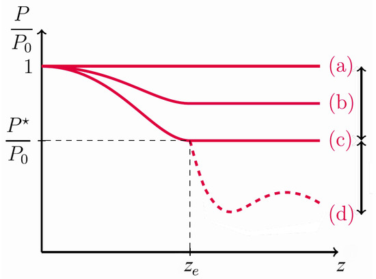
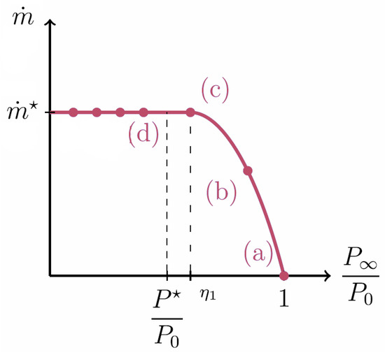
Figure 1 and Figure 2 report the pressure ratio and the mass flow rate evolution as a function of the axial distance for a convergent nozzle.

Figure 1.

Pressure evolution along nozzle axis for various pressure ratios.

Figure 2.

Mass flow rate for various pressure ratios.

The first regime depicts a subsonic flow (cases a and b); the mass flow increases as the downstream pressure decreases, and the exit pressure is equal to the ambient one. Critical conditions are reached if the upstream pressure increases and the nozzle is choked (cases c and d). The outflow pressure is equal to the critical pressure (

P^{*}

), and the mass flow cannot increase more; it is called indeed choked as reported in Figure 2.

It follows that, an the exit section, the pressure is greater than the ambient one and to achieve pressure equilibrium, under-expanded jets arise.

In choked conditions, the pressure waves cannot travel back upstream, and the mass flow rate is no longer dependent on downstream conditions (

{\dot{m}}^{*}

). The flow characteristics inside the nozzle, in fact, only depend only on the upstream boundary conditions.

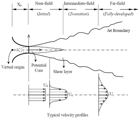
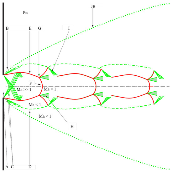
As represented in Figure 3, it is common practice to divide the jet into three zones ^[1][29]:

Figure 3.

Under-expanded jet zones.

the near-nozzle zone;
the transition zone;
the far-field zone;

The near-nozzle zone is split into two sections: the core and the mixing layer. In the former, also called the gas-dynamic area, the flow is separated from the environment, and its behaviour is governed mostly by compressible effects and is rather steady. The fluid expands iso-entropically until it is re-compressed by shock waves.

In the mixing layer, turbulence causes an interaction between the injected fluid and the surrounding environment, which is characterized by huge turbulent structures (vortices) that are formed within the fluid flow downstream of the nozzle outlet. A shearing zone between the frontier of the potential core of the jet and the constant pressure line can be distinguished.

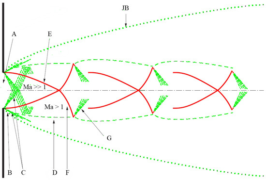
Depending on the pressure ratio, different under-expanded jet configurations can be observed in the near-nozzle zone:

The jet is weakly under-expanded, a normal shock appears in the exit plane.
[34,35]. As depicted in Figure 6, the structure is dominated by a unique barrel. In this case, the Mach disc is no longer considered as a normal shock, and its curvature must be considered. Due to the momentum exchange generated by the ambient fluid’s entrainment, the jet’s overall diameter will decrease, resulting in an extremely long plume.

The jet is moderately under-expanded and has a “diamond” or “X” structure, depicted in Figure 4, $2 < η_{0} < 4$ ^[2]^[3]. In the exit plane (marker A), a Prandtl–Meyer expansion fan (marker C) expands the fluid downstream of the device’s edges up to the jet boundary that corresponds to the external surface of the mixing layer (marked JB). The expansion waves are reflected as compression waves when they reach the constant pressure streamline (marker D), where the pressure matches the ambient pressure. They converge on the inner jet and merge to produce an oblique shock (marker E), commonly referred to as the intercepting shock.

The jet is highly under-expanded, $4 < η_{0} < 7$ ^[4][5]. It has a “barrel” or “bottle” structure, shown in Figure 5, Mach disc appears (due to a singular reflection). When the pressure ratio grows, the regular reflection of the intercepting shock on the axis is no longer possible. As a result, above the critical angle, this reflection becomes singular, resulting in the appearance of a normal shock-denominated Mach disc (marker F). The triple point is defined as the intersection of the intercepting shock, the Mach disc and the reflected shock (marker G). A slipstream (marker H) develops at this point: this is an embedded shear layer that divides the flow upstream of the Mach disc (subsonic) from the flow downstream of the reflected shock (supersonic).[30,31]. In the exit plane (marker A), a Prandtl–Meyer expansion fan (marker C) expands the fluid downstream of the device’s edges up to the jet boundary that corresponds to the external surface of the mixing layer (marked JB). The expansion waves are reflected as compression waves when they reach the constant pressure streamline (marker D), where the pressure matches the ambient pressure. They converge on the inner jet and merge to produce an oblique shock (marker E), commonly referred to as the intercepting shock.
The jet is extremely (or very highly) under-expanded, $η_{0} > 7$ ^[6][7]. As depicted in Figure 6, the structure is dominated by a unique barrel. In this case, the Mach disc is no longer considered as a normal shock, and its curvature must be considered. Due to the momentum exchange generated by the ambient fluid’s entrainment, the jet’s overall diameter will decrease, resulting in an extremely long plume. $4 < η_{0} < 7$
[32,33]. It has a “barrel” or “bottle” structure, shown in Figure 5, Mach disc appears (due to a singular reflection). When the pressure ratio grows, the regular reflection of the intercepting shock on the axis is no longer possible. As a result, above the critical angle, this reflection becomes singular, resulting in the appearance of a normal shock-denominated Mach disc (marker F). The triple point is defined as the intersection of the intercepting shock, the Mach disc and the reflected shock (marker G). A slipstream (marker H) develops at this point: this is an embedded shear layer that divides the flow upstream of the Mach disc (subsonic) from the flow downstream of the reflected shock (supersonic).

The jet is extremely (or very highly) under-expanded, $η_{0} > 7$

Figure 4.

Structure of a moderately under-expanded jet.

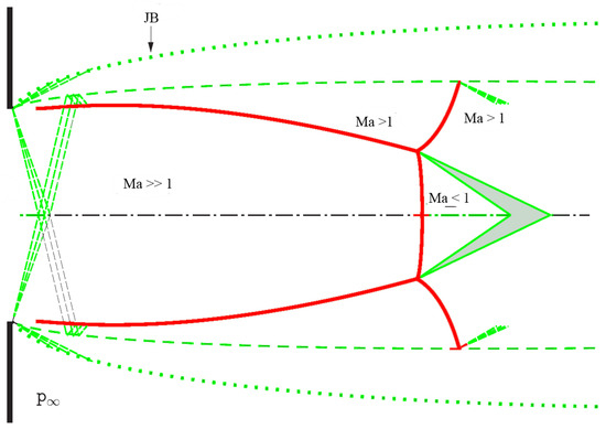
Figure 5.

Structure of a highly under-expanded jet.

Figure 6.

Structure of a very highly under-expanded jet.

Nevertheless, the Mach disc is undoubtedly one of the most studied features of under-expanded jets Moreover, there is still significant ongoing discussion regarding the transition from a regular reflection to a singular reflection, accompanied by the appearance of the Mach disc. This phenomenon is currently quantitatively not well known, particularly the dependence (and interactions) on pressure range and exit Mach number, fluid characteristics (i.e., the polytropic coefficient), nozzle shape, and exit nozzle angle ^[8][36].

The Mach disc location is primarily governed by the pressure ratio, increases with the Mach number and, among the many, a good estimation of the position is given by the following relation:

\frac{H_{d}}{D} = 0.67 \sqrt{η_{0}}

with $H_{d}$ Mach disc height, D outlet section diameter ^[6][8][9].

Mach disc height, D outlet section diameter [34,36,37].

The Mach disc width or diameter was clearly less investigated than the Mach disc length. However, it appears that it is also mainly governed by the pressure ratio and strongly dependent on the nozzle geometry and shape ^[10][11][12][38,39,40].

Towards the end of the near-nozzle zone, the sonic line reaches the axis, indicating that the mixing layer has fully replaced the inner region. This marks the beginning of the transition zone, where variations in variables, both longitudinally and radially, become minimal. In this region, a more effective mixing of the two fluids, the ejected fluid and the ambient fluid, takes place. As a result, the pressure field becomes more homogenized as entrainment occurs throughout the transition zone.

In the far-field zone, the jet exhibits self-similarity, but compressible effects may still be present if the Mach number is above 0.3 and may even be supersonic. Qualitatively, the normalized radial profiles of the mean variables follow the same pattern, typically characterized by a Gaussian profile.

2. Experimental Observation of Under-Expanded Jets

The observation of under-expanded jets can be performed both with quantitative and qualitative techniques. Among the first category, schlieren and shadowgraph imaging surely can be mentioned, adopted for capturing images of both near and far field zones ^{[13][14][15][16]}[13,41,42,43].

High-speed schlieren imaging is a robust diagnostic technique capable of visualizing optical in-homogeneities of transparent media, otherwise not visible to the human eye ^[17][18][19][44,45,46]. The method is sensitive to changes in the refractive index of a light beam travelling through a heterogeneous medium. 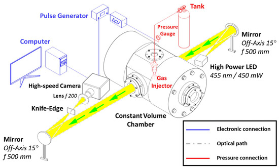For this reason, Schlieren diagnostic is frequently adopted for the observation of compressible flows, such as under-expanded jets, in which the difference in refractive index is caused by the gradient of density between the injected fuel and the ambient gas ^[17][44].

Figure 7 shows the schematic diagram of a typical experimental setup for schlieren imaging.

The Schlieren light source is usually a high-power LED lamp. A series of lenses and glasses modify the beam characteristics. The main difference between Schlieren and shadowgraph is the presence of a knife-edge in the first case to regulate the percent of light cutoff, obtaining the desired contrast for the Schlieren images. High-speed cameras are adopted for recording images with frame rates of the order of thousands of frames per second. Depending on the magnification system, different spatial resolutions can be achieved.

The injection system usually consists of a pressurized fuel tank, a pressure transducer and a pressure regulator to ensure the desired value for the test conditions. The transistor–transistor logic (TTL) triggering signal produced by a pulse generator is used by an Electronic Control Unit (ECU) to control the injection events and to guarantee proper synchronization and delay between the injection and acquisition chain.

Under-expanded jets are almost always being observed in Constant Volume Chambers (CVC), optically accessible through quartz windows with the injector fixed in a customized holder.

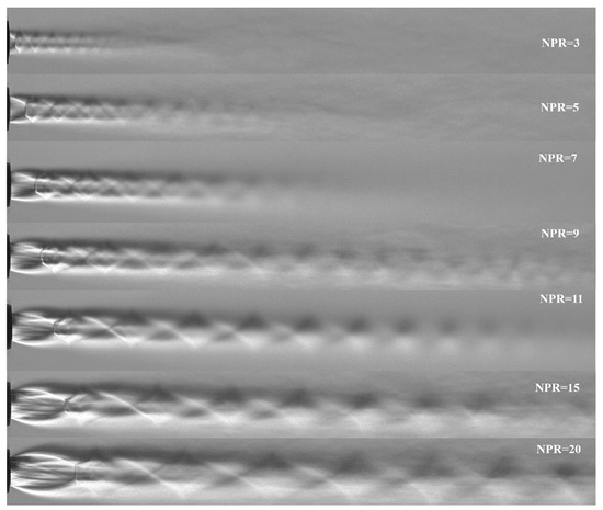
The images recorded with these techniques provide a proficient visualization of the near field zone, and so of the barrel shocks, the Mach discs, etc., as well as the overall spray structure, allowing the evaluation of macroscopic parameters such as the Mach disc height, width, the jet tip penetration, the jet angle, the volumetric growth, the tip speed, radial expansion, etc. Figure 8 depicts some classical visualization of the under-expanded jets obtained with schlieren imaging and regarding various jet’s characteristics [48].

These information are of relevant importance for verifying and validating CFD simulation codes by comparison of the aforementioned parameters but, at the same time, do not allow to evaluate microscopic features of the jet or give a quantitative estimation of local fuel concentration, jet temperature or velocity. To obtain some of these information other experimental techniques are required. They are Planar Laser-Induced Fluorescence (PLIF) or Particle Image Velocimetry (PIV) ^{[16][22][23][24][25][26]}[43,49,50,51,52,53].

The PIV technique is a non-intrusive diagnostic technique that allows the velocity field to be measured on a two-dimensional plane. The measurement principle is based on determining the distance the tracer particles cover in a known time interval ^[27][28][54,55]. The typical elements of a PIV system are a laser source (typically a pulsed Nd-YAG laser with a wavelength of 532 nm), an optical system, a camera and a data acquisition system (DAQ).

The PLIF technique allows the measurement of the concentration of species and the temperature in the flow field of a fluid. It is based on the process of photon absorption–emission, and therefore, on the phenomenon of natural fluorescence of molecules and atoms. Through the PLIF technique, it is possible to obtain visualization with high spatio-temporal resolution. Although the instantaneous (temporally based) quantitative measurement of the parameters of interest remains complex, it is still possible to obtain quantitative measurements of concentration, temperature, pressure and speed based on an average of consecutive sequences (time-averaged).

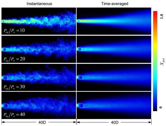
Figure 9 depicts some results regarding the fuel concentration of under-expanded jets [53].

Figure 9. Visualization of under-expanded jets by means of PLIF optical technique for different

P_{i n j} / P_{a m b}

3. CFD Simulation of Under-Expanded Jets

Computational fluid dynamic codes (CFD) are undoubtedly the other powerful tool broadly adopted to investigate under-expanded jets. The advantages of developing a virtual model of this engineering problem are quite obvious not only to understand the underlying physics of these flows but also with the perspective of the application to the propulsion system.

This paragraph aims to illustrate, in a synthetic but also organized fashion, the main characteristics of the CFD codes used by researchers to study the aforementioned problem. Further than in-house developed codes, basically three finite volume CFD codes were used. They are OpenFOAM, CONVERGE and STAR-CCM+ ^[29][30][31][59,60,61]. It should also be mentioned that some studies use the Lattice Boltzmann method ^[32][33][62,63]. The following two sub-sections report the main characteristics of the discretization schemes adopted and of the turbulence modelling selected.

3.1. Discretization Schemes and Solution Algorithms

The simulation of under-expanded jets requires the adoption of high-order numerical schemes able to describe flow-field discontinuities along with avoiding undesired oscillations. High-order schemes are required both for spatial discretization and temporal integration.

Methodologies, based on Riemann solvers, such as the Weighted Essentially Non-Oscillatory schemes (WENO) or the Piecewise Parabolic Method (PPM), give the best reproduction of compressible flow but have relevant limitations. These approaches involve characteristic decomposition and Jacobian evaluation, and so they were implemented only for structured grids. The adaptive central-upwind sixth-order weighted essentially non-oscillatory (WENO-CU6) scheme with low dissipation was used by Ren Z et al. ^[34][64] to achieve a proper resolution of the flow properties around the shock waves. Seventh-order accurate weighted essentially non-oscillatory (WENO7) reconstruction of the characteristic fluxes was also adopted for simulating under-expanded jets. The shocks and discontinuities can be resolved using highly accurate and low-dissipation hybrid ENO schemes with shock detectors ^[35][36][37][65,66,67].

Contrarily, unstructured grids are far more flexible than structured grids and can easily discretize complex geometries ^[38][39][40][68,69,70]. One of the principal methods developed for unstructured grids uses the so-called central schemes formulations of Kurganov (KNP) and Kurganov and Tadmor (KT) ^[41][42][71,72]. These are non-staggered second-order central methods that use the cell centres’ values to evaluate the cell faces’ fluxes. The cell-to-face flow interpolation is divided into inward and outward directions with respect to the face owner cell. An extensive and detailed description can be found in ^[38][68]. Considering the intrinsic geometrical complexity of the injector’s nozzles, these schemes are broadly adopted for this kind of simulation in union with flux limiters of Minmod or of Van Leer to ensure stability and convergence of the computation ^[38][43][68,73]. This discretization method, initially implemented in OpenFOAM’s solver

r h o C e n t r a l F o a m

, was exploited in various other solvers purposely developed to study under-expanded jets ^{[44][45][46][47][48][49][50]}[74,75,76,77,78,79,80]. Another proficient scheme used is the Advection Upstream Splitting Method (AUSM⁺-up). AUSM+-up is accurate and reliable in solving fluid flows with any arbitrary range of velocities, but it excels at high-velocity flows with strong discontinuities like shock waves ^[51][52][81,82]. AUSM+-up avoids explicit artificial dissipation by using a separate splitting for the pressure terms of the governing equations; the mass flux and pressure flux are calculated on the basis of local flow characteristics (including the speed of sound) to ensure precise information propagation inside the fluid for convective and acoustic processes ^[53][83]. This minimizes numerical dissipation, especially in high-velocity flows, and prevents wiggles at flow discontinuities like shocks.

The solution methods commonly used involve both explicit (density-based) ^[54][55][56][84,85,86] and Pressure Implicit Split Operator (PISO) algorithms ^{[57][58][59][60][61]}[56,87,88,89,90]. The density-based approach proved to be the best choice for reproducing under-expanded jet features. Implicit (or pressure-based) methods for solving fluid-flow governing equations were historically employed for incompressible flows and only recently adapted to account for compressible flows. However, as broadly demonstrated in the literature ^{[54][55][56][60]}[84,85,86,89], the best choice in terms of results accuracy is represented by explicit methods (or density-based). The reason for that is intrinsically contained in the algorithm procedure. The temporal integration is usually performed using high-order schemes such as explicit Runge–Kutta 4th (RK4) ^[54][84].

Another relevant aspect of under-expanded jet simulation is the computation of the thermo-physical properties for the species involved in the fluid flow. The equation of state (EoS) (for a description of the pressure–volume–temperature (P-V-T) relationship) is crucial to the accuracy of the solution. Further than the ideal-gas EoS, Cubic EoS such as Soave–Redlich–Kwong (SRK) and Peng–Robinson (PR) were widely applied due to their simplicity and reasonable accuracy ^{[31][46][47][57][62][63][64][65]}[56,61,76,77,91,92,93,94].

3.2. Turbulence Modelling

The numerical solution of the fluid-dynamic problem is valid when the computational grid is fine enough to resolve all the flow scales ^[55][85]. This would be a Direct Numerical Simulation (DNS) of the flow, which is now unaffordable due to its complexity and resource demands. So, turbulence modelling techniques, such as Reynolds Averaged Navier Stokes (RANS) or Large Eddy Simulation (LES), are preferred for under-expanded jet simulations ^{[48][55][56][66]}[78,85,86,95].

Among the many simulation approaches regarding under-expanded jets, just a few use RANS, while most adopt LES models. The LES technique is based on modelling the lower scales, which are universal and unaffected by flow geometry, while explicitly solving the larger ones. This is done by mathematically filtering the governing equations and introducing the Sub-Grid Stress (SGS) tensor (

τ_{s g s}

) ^[67][96]. The SGS term modelling involves an eddy viscosity approximation. Various SGS closure models can be found in the literature. In some cases, LES WALE model is used, both without wall functions or applying global damping functions. The model produces an efficient and fast-solving scheme due to its algebraic formulation. This approach also showed some promising results in predicting the transition from laminar to turbulent regimes ^[68][97].

The Yoshizawa model is another common choice. It is a one-equation eddy viscosity model for compressible flows ^[69][70][98,99], which is different from zero equation models such as the Smagorisky model. It exploits a transport equation to compute the local SGS kinetic energy

k_{s g s}

. Then, the sub-grid scale eddy viscosity

ν_{s g s}

is calculated using the

k_{s g s}

field and the filter dimension

Δ

(usually evaluated from the grid size) according to the following relation:

ν_{s g s = C_{k} Δ \sqrt{k_{s g s \sqrt{}}}}

where $C_{k}$ is a model constant whose default value is 0.094.

is a model constant whose default value is 0.094.

The scale selective discretization (SSD) technique proposed by Vuorinen et al. relates to the so-called implicit LES (ILES) modelling category ^{[54][71][72][73]}[84,100,101,102]. However, unlike ILES, the SSD approach targets the dissipative effects exclusively to the flow’s smallest scales via scale separation procedure. A Laplacian filter separates the scales by splitting the convection term into low and high-frequency components for which centred and upwind-biased techniques can be used individually.