System identification, as the name suggests, is the process of identifying a system behavior by means of its measured or observed input and output data ^[1][22]. Through different algorithms that are based on numerical optimization, the relationship between the system input and output is mapped during identification ^[2][1].

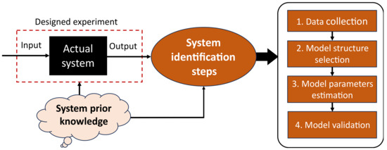
As illustrated in Figure 1, system identification involves four main steps: data collection or acquisition, model structure definition or selection, model parameters estimation, and model validation ^[3][4][2,23]. The first step involves getting input–output data from the physical system by designing and conducting an experiment covering the system’s operating limits/bounds. It is crucial to acknowledge that the obtained dataset could have outliers and this necessitates data-prepossessing operations such as normalization, resampling, or filtering. Secondly, a model structure such as transfer function, state-space, autoregressive with exogenous (ARX), or neural network is selected depending on the available insight or prior knowledge of the system under consideration. In the third step, the model parameters are trained or estimated using different algorithms like LS or backpropagation. During estimation, the model parameters act as a driver and play the role of driving the model, thereby fitting its response to match that of the actual system. The fourth and last step is to validate the estimated model. This is performed to guarantee that the developed model will serve the intended application (e.g., control or fault detection). In a scenario where the developed model turns out to be unsatisfactory, the identification process is reworked (i.e., performed all over again) ^[3][5][2,4]. For this reason, system identification is regarded as an iterative process and it involves the user trying out different choices in terms of the model structure and even the estimation algorithm to arrive at the best model.

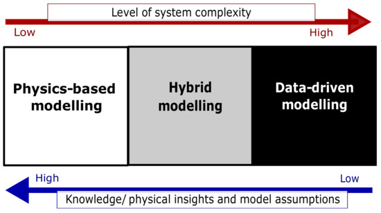
There are three main modeling approaches: physics-based, data-driven, and hybrid modeling.

• Physics-based modeling: This method utilizes knowledge of the underlying physical laws governing the system’s behavior. The equations and parameters are theoretically determined and solved ^[2][1]. However, in reality, a purely physics-based model is impractical for large-scale or complex systems ^[6][7][24,25]. The model developed through this approach is referred to as a mathematical one;
• Data-driven modeling: This method is suitable for complex nonlinear systems where little or no knowledge of their governing physical laws exists. The model structure and parameters are unknown, and the model architecture is not based on physical laws. As a result, the parameters often lack physical meaning or interpretation ^[2][8][1,26]. The model developed through this approach is known as data-driven or intelligent;
• Hybrid modeling: In this case, partial knowledge about the system is available. The model structure is either fully or partially known, and its parameters are estimated using system data ^[2][9][1,27]. The resulting model is called hybrid or physics-informed data-driven.

The three modeling approaches are depicted in Figure 2. The upper arrow indicates increasing complexity, while the lower arrow indicates the direction of increasing knowledge and model assumptions according to the modeling methods.

The modeling problems posed by dynamical systems can be classified into forward and inverse problems. The forward modeling problem involves computing a system response or solution given its mathematical model and parameters ^[10][28]. In forward problems, ordinary differential and partial differential equations (ODEs and PDEs) are solved analytically or numerically using the Euler method, Runge–Kutta method, finite element method, finite difference method, and so on. In contrast, the inverse modeling problem involves the estimation of unknown model parameters that would give a small prediction error when compared to the output data observed from a physical system ^[11][29]. The parameters can be identified (estimated) using various algorithms such as least squares (LS) ^[12][30], recursive least squares (RLS) ^[13][31], the genetic algorithm (GA) ^[14][32], NNs ^[15][33], etc.

The concept of identifying the model parameters of a system is known as parameter identification, and this topic can be viewed as an inverse modeling problem. Parameter identification is performed either online or offline. In online parameter identification, model parameters are estimated in real time with the help of algorithms such as RLS ^[12][16][30,34] and the extended Kalman filter ^[17][18][35,36], as new sensor data are available from the physical system. On the other hand, offline parameter identification is conducted by acquiring input–output data from the system, storing the data, and then using an algorithm like LS or GA to estimate the unique parameters of the system. In Table 1, the two-parameter identification methods are compared in terms of the type of parametric results they give, the ease of data preprocessing, and the computational power and storage demands.

In mechatronic systems, such as pendulums, DC motors, and mass-damper setups, modeling can be accomplished using either first principles or physical laws. However, achieving accurate models often requires identifying the system’s parameters. One major challenge is accurately representing the impact of friction, a nonlinear phenomenon that affects the efficiency of these systems ^[19][20][37,38].

Friction models can be categorized into static and dynamic models. Static models assume no relative motion during standstill (resting friction phase) and describe the relationship between friction force and relative velocity. On the other hand, dynamic models capture the features of presliding and sliding regions, including their transition effects ^[21][39].

Static models consist of Coulomb friction, viscous friction, the Stribeck effect, Karnopp, and Armstrong. Moreover, dynamic models include Dahl, LuGre, Leuven, and bristle friction models ^{[22][23][24][25]}[40,41,42,43].

Applying an accurate friction model can facilitate friction compensation, helping to prevent issues such as slow responses, tracking errors, stick-slip motion, and limit cycles ^[26][27][44,45]. Notably, for dynamic systems developed purely through data-driven approaches, a separate friction model is unnecessary, as frictional losses are already accounted for in the experimental data used to build the model.