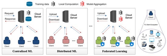
Federated learning (FL) is a rapidly growing field that enables multiple clients to train a machine learning model while preserving their data privacy [1]. It has been extensively used in various fields, including healthcare, finance, and social media, where privacy is critical ^[2][3][2,3]. In FL, the clients (devices) perform local training on their respective datasets and then share only the model updates with the server, aggregating the updates to generate a global model [4]. In contrast to conventional centralized machine learning, federated learning (FL) and distributed machine learning offer unique mechanisms for training models across decentralized devices or data sources. However, it is FL that emphasizes collaborative model training with a keen focus on preserving data privacy, minimizing communication overheads, and catering to dynamic and potentially heterogeneous data environments. Distributed machine learning, while reducing computational constraints through parallel processing, often involves more frequent data exchanges without the inherent privacy-preserving design of FL [5]. Figure 1 provides a comprehensive architectural comparison of FL against the traditional centralized and distributed machine learning frameworks. It showcases the nuances in data distribution, model updates, and communication patterns among these paradigms, thus emphasizing the distinct attributes and advantages of FL.

FL is a revolutionary approach in distributed machine learning, promising enhanced data privacy and decentralized model training [6]. However, the communication overheads associated with FL have emerged as a considerable challenge, especially when they pertain to scalability and efficiency. In the FL paradigm, communication costs are bifurcated into two primary categories: upload and download costs. The former encapsulates the data transmitted by clients to the server during the training phase, while the latter accounts for data fetched from the server by the clients [7]. Notably, these costs are influenced by various parameters, such as the dataset size, model intricacy, client count, and network bandwidth ^[8][9][8,9].

The ramifications of these communication costs on FL’s efficiency have been the subject of intensive research. Empirical analyses have ascertained that communication costs can act as substantial constraints, inhibiting the scalability and effectiveness of FL systems ^[10][11][10,11]. To combat these challenges, innovative solutions, such as compression methodologies and model quantization, have been postulated ^[12][13][12,13]. Compression solutions primarily focus on diminishing the magnitude of model updates, thus curtailing upload expenses, whereas model quantization optimizes model parameters’ precision, facilitating further reductions in upload costs.

Moreover, the aspiration for energy-efficient communication systems is a pressing concern that complements the drive for communication efficiency [14]. Reducing communication overheads through FL directly ties into energy savings. Given that every data exchange involves energy consumption, optimizing the FL process impacts the bandwidth and potentially contributes to reduced energy expenditures, a vital consideration for modern communication networks ^[15][16][15,16]. FL’s capacity to minimize data transmission inherently reduces energy consumption, placing it at the forefront of strategies to develop energy-efficient communication networks.

2. Fundamentals of Federated Learning

Table 12 provides a description of the fundamentals of FL, including the advantages and challenges associated with FL. The fundamentals are the following:

• Decentralized data: FL involves multiple clients or devices that hold their respective data. As a result, the data are decentralized and not stored in a central location ^[17][18][32,33]. This decentralized nature of data in FL helps preserve the local data’s privacy, but it can also lead to increased communication costs ^[19][34]. The decentralized data distribution means more data must be transferred between the clients and the central server during the training process, leading to higher communication costs ^[20][35].
• Local model training: FL allows each client to perform local model training on its respective data. This local training ensures that the privacy of the local data is preserved, but it can also lead to increased communication costs ^[21][36]. The local model updates need to be sent to the central server, which aggregates them to generate a global model. The communication costs of sending these updates to the central server can be significant, particularly when the number of clients or data size is large ^[22][23][37,38].

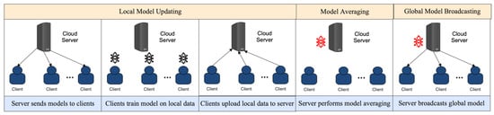
Figure 23 delves into the intricacies of the FL communication protocol. Beyond merely illustrating the flow, it captures the iterative nature of client–server interactions, highlighting the stages where communication overheads might arise and emphasizing the importance of efficient data exchanges in the FL process. 

 

3.1. Local Model Updating

Local model updating (LMU) is one of the key techniques used in FL to overcome communication deficiency ^[35][65]. In LMU, each participating device trains the shared model on its local data, and only the updated parameters are sent to the central server for aggregation ^[36][37][66,67]. This approach significantly reduces the amount of data that needs to be transmitted over the network, thereby reducing communication costs and latency. However, several factors can affect the performance of LMU in FL, including the quality and quantity of local data, the frequency of updates, and the selection of participating devices. Below, some of these factors and their impact on the communication efficiency of LMU in FL are discussed:

• Quality and quantity of local data: The quality and quantity of local data available on each participating device can significantly impact the performance of LMU in FL. If the local data are noisy or unrepresentative of the global dataset, it can lead to a poor model performance and increased communication costs ^[38][39][68,69].
• Frequency of updates: The frequency of updates refers to how often the participating devices send their updated parameters to the central server for aggregation ^[40][41][42][73,74,75]. A higher frequency of updates can lead to faster convergence and an improved model performance but can also increase communication costs and latency.
• Model aggregation: After the local model training is completed, the clients send their model updates to the central server for aggregation ^[24][25][39,40]. The server aggregates the model updates to generate a global model, which reflects the characteristics of the data from all the clients ^[26][41]. The model aggregation process can lead to significant communication costs, particularly when the size of the model updates is large or the number of clients is high ^[27][28][29][22,42,43].
• Selection of participating devices: The selection of participating devices in FL can significantly impact the performance of LMU ^[43][44][49,78]. If the participating devices are too few or diverse, it can lead to poor model generalization and increased communication costs. 
  Privacy preservation: FL is designed to preserve the privacy of the local data, but it can also lead to increased communication costs ^[30][31][44,45]. The privacy-preserving nature of FL means that the local data remain on the clients, and only the model updates are shared with the central server ^[32][46]. However, this also means more data must be transferred between the clients and the server during the training process, leading to higher communication costs.

Category	Description
Definition	FL is a machine learning setting where the goal is to train a model across multiple decentralized edge devices or servers holding local data samples, without explicitly exchanging data samples.
Key Components	The main elements of FL include the client devices holding local data, the central server that coordinates the learning process, and the machine learning models being trained.
Workflow	The typical FL cycle is as follows: (1) The server initializes the model and sends it to the clients; (2) Each client trains the model locally using its data; (3) The clients send their locally updated models or gradients to the server; (4) The server aggregates the received models (typically by averaging); (5) Steps 2–4 are repeated until convergence.
Advantages	The benefits of FL include (1) privacy preservation, as raw data remain on the client; (2) a reduction in bandwidth usage, as only model updates are transferred, not the data; (3) the potential for personalized models, as models can learn from local data patterns.
Challenges	FL faces several challenges, including (1) communication efficiency; (2) heterogeneity in terms of computation and data distribution across clients; (3) statistical challenges due to non-iid data; (4) privacy and security concerns.
Communication Efficiency Techniques	Communication efficiency can be improved using techniques, such as (1) federated averaging, which reduces the number of communication rounds; (2) model compression techniques, which reduce the size of model updates; (3) the use of parameter quantization or sparsification.
Data Distribution	In FL, data are typically distributed in a non-iid manner across clients due to the nature of edge devices. This unique distribution can lead to statistical challenges and influence the final model’s performance.
Evaluation Metrics	Evaluation of FL models considers several metrics: (1) global accuracy, measuring how well the model performs on the entire data distribution; (2) local accuracy, measuring performance on individual client’s data; (3) communication rounds, indicating the number of training iterations; (4) data efficiency, which considers the amount of data needed to reach a certain level of accuracy.

3. Communication Deficiency

The communication deficiency of FL is an important issue that needs to be addressed for this type of distributed machine learning to be successful. In FL, each client, typically a mobile device, must communicate with a centralized server to send and receive updates to the model ^[33][47]. As the number of clients increases, the amount of communication between the server and clients increases exponentially. This can become a major bottleneck, causing the training process to be slow and inefficient. Additionally, communication can be expensive, especially for mobile devices, so minimizing the amount of communication required for FL is important ^[34][48].

3.2. Model Averaging

Model averaging is a popular technique used in FL to overcome the communication deficiency problem ^[45][81]. In particular, model averaging involves training multiple models on different devices and then combining the models to generate a final model that is more accurate than any individual model ^[46][82]. The model averaging technique involves training multiple models using the same training data on different devices. Each device trains its own model using its local data, and the models are then combined to generate a final model that is more accurate than any individual model ^[47][48][83,84]. The models are combined by taking the average of the weights of the individual models. This technique is known as “Weighted Average Federated Learning” ^[49][85].

3.3. Broadcasting the Global Model

Global model broadcasting is a crucial step in FL, where the locally trained models are aggregated to form a global model ^[50][93]. The global model represents the collective knowledge of all the edge devices and is used for making predictions and decisions. The global model must be communicated efficiently and effectively across all devices to achieve a high accuracy and high convergence rate ^[51][94]. However, this can be challenging in the presence of communication deficiency. In the parameter-server-based approach, a central server acts as a parameter server, which stores and manages the model parameters. The edge devices communicate with the parameter server to upload their local model updates and download the new global model ^[52][97]. The parameter server can update the global model by using a synchronous or asynchronous approach. In the synchronous approach, the edge devices upload their local model updates at regular intervals, and the parameter server updates the global model after receiving updates from all devices. In the peer-to-peer approach, the edge devices communicate with each other directly to exchange their local model updates ^[53][54][98,99]. The devices can either use a fully connected topology or a decentralized topology to exchange their model updates. Communication deficiency is a major challenge in global model broadcasting in FL. The deficiency can be caused by a limited bandwidth, high latency, or network congestion ^[55][56][100,101]. The impact of communication deficiency can be severe, leading to slow convergence, a low accuracy, and even a divergence of the global model. In particular, a limited bandwidth can restrict the amount of data that can be transmitted between the edge devices and the central server. This can result in delayed model updates and slower convergence of the global model.

4. Resource Management

Managing resources is critical for the success of FL, which relies on a network of devices to train a machine learning model collaboratively ^[57][109]. In addition to computational and communication resources, the availability and quality of edge and server resources can significantly impact the performance of FL systems. Table 24 shows the categorization of FL resources in terms of the edge and server. In addition, Figure 34 distinctly portrays the myriad techniques deployed for both client and server resource management in the context of federated learning.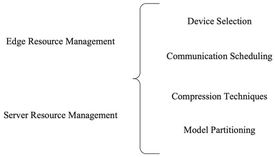

 

Resource	Edge Resource	Server Resource
Data Storage	Local Storage	Distributed Storage
Data Aggregation	Local Aggregation	Distributed Aggregation
Data Processing	Local Processing	Cloud Processing
Data Security	Local Encryption	Cloud Encryption

4.1. Edge Resource Management

Edge resources refer to the computing and storage resources available on devices participating in the FL process. Edge devices typically have limited resources compared to cloud servers, which makes managing these resources a critical task in FL ^[58][110]. Effective edge resource management can help reduce communication costs and improve the overall performance of the FL system.

4.1.1. Device Selection

The first step in edge resource management is selecting appropriate devices for FL. Edge devices include smartphones, tablets, sensors, and other IoT devices. These devices vary in their processing power, memory capacity, battery life, and network connectivity. Therefore, selecting appropriate edge devices is critical for ensuring efficient resource management in FL ^[59][111]. One way to select edge devices is based on their processing power. Devices with more processing power can handle more complex machine learning models and computations ^[60][64]. However, devices with more processing power also tend to consume more energy, which can limit their battery life. Network connectivity is another important factor to consider when selecting edge devices. Devices with reliable and high-speed network connectivity can communicate with the central server more efficiently, while devices with poor connectivity may experience delays or errors during communication ^[61][62][114,115]. 

4.1.2. Communication Scheduling

Communication scheduling is another important aspect of edge resource management in FL. Communication refers to exchanging data and models between edge devices and the central server ^[63][64][62,116]. Communication scheduling involves deciding when and how frequently to communicate and which devices to communicate with. One strategy for communication scheduling is to schedule communication based on the availability and capacity of the edge devices. Devices with limited resources can be scheduled to communicate less frequently, while devices with more resources can be scheduled to communicate more frequently. This approach can help reduce the overall communication costs of the FL system ^[65][117].

4.1.3. Compression Techniques

Compression techniques are important for managing edge resources in FL. In particular, compression techniques involve reducing the data size and exchanging models between edge devices and the central server without sacrificing model accuracy ^[66][120]. The need for compression arises due to the limited resources available on edge devices. Edge devices typically have a limited storage capacity and network bandwidth, making transmitting large amounts of data and models challenging ^[67][121]. Compression techniques can help reduce the amount of data and models transmitted, making performing FL on edge devices with limited resources possible. There are several techniques for compressing data and models in FL. One common technique is quantization, which involves reducing the precision of the data and models ^[68][122].

4.1.4. Model Partitioning

Model partitioning is another critical component of FL systems, as it involves dividing the machine learning model into smaller submodels that can be trained on individual devices. Model partitioning aims to reduce the amount of communication required between devices while ensuring that the model’s overall accuracy is not compromised ^[69][128]. Several strategies have been developed for model partitioning in FL systems. One common approach is vertical partitioning, where the model is divided based on the features or attributes being used ^[70][129]. For example, in an image recognition model, one device may be responsible for training the feature extraction layer, while another device may train the classification layer. This approach can be particularly useful when the model has many features, allowing the devices to focus on a subset of the features ^[71][130].

4.2. Server Resource Management

Server resource management is a crucial aspect of FL that is responsible for optimizing the utilization of server resources to enhance the efficiency and accuracy of FL models ^[72][73][134,135]. A server’s role in FL is coordinating and managing communication and computation among the participating edge devices. The server needs to allocate computational and communication resources optimally to ensure that the participating devices’ requirements are met while minimizing the communication costs and enhancing the FL model’s accuracy.

4.2.1. Device Selection

Device selection is a critical aspect of server resource management in FL. In an FL system, edge devices train a local model using their data and then communicate the model updates to the server ^[74][75][136,137]. The server aggregates the updates from all devices to create a global model. However, not all devices are suitable for participating in FL for several reasons, such as a low battery life, poor network connectivity, or low computation power. Therefore, the server must select the most suitable devices to participate in FL to optimize resource utilization and enhance model accuracy ^[76][138].

4.2.2. Communication Scheduling

The server needs to allocate communication resources optimally to ensure that the participating devices’ updates are timely while minimizing communication costs. In FL, devices communicate with the server over wireless networks, which are prone to communication delays, packet losses, and network congestion ^[77][140]. Therefore, the server must effectively schedule communication between devices and the server. The communication schedule can be based on several factors, such as the device availability, network congestion, and data priority.

4.2.3. Compression Techniques

In FL, the server receives updates from all participating devices, which can be significant in size. The size of the updates can be reduced by applying compression techniques to the updates before sending them to the server. Compression reduces the communication and the server’s computational costs ^[78][142]. The compression techniques can be based on several factors, such as the update’s sparsity, the update’s structure, and the update’s importance.

4.2.4. Model Partitioning

The model partitioning can be based on several factors, such as the model’s size, the model’s complexity, and the available server resources ^[79][143]. A popular model partitioning approach is the model distillation technique, which distills the global model into a smaller submodel ^[80][144].

5. Client Selection

5.1. Device Heterogeneity

Device heterogeneity refers to the variety of devices and their characteristics that participate in an FL system. The heterogeneity of devices presents several challenges in FL, including system heterogeneity, statistical heterogeneity, and non-iid-ness ^[81][148].

5.1.1. System Heterogeneity

System heterogeneity refers to differences in the hardware, software, and networking capabilities of the devices participating in the FL system. The heterogeneity of these devices can lead to significant performance disparities and make it difficult to distribute and balance the workload among the devices ^[82][149]. These discrepancies can cause communication and synchronization issues, leading to slow convergence rates and increased communication costs.

5.1.2. Statistical Heterogeneity

Statistical heterogeneity refers to the differences in the data distributions across the devices participating in the FL system. In an ideal FL system, the data should be identically and independently distributed (IID) across all devices, allowing the global model to be trained effectively ^[83][84][153,154]. However, in practice, the data are often non-IID, which can lead to a poor model performance.

5.1.3. Non-IID-Ness

Non-iid-ness refers to the situation where the data distribution across the devices significantly differs from the global distribution. This is a common challenge in FL scenarios, where devices may collect data from different sources or have unique user behavior patterns ^[85][157]. The presence of non-iid-ness can lead to slower convergence rates and a poor model performance, as the global model may not accurately represent the data distribution across all devices ^[86][87][21,158].

5.2. Device Adaptivity

5.2.1. Flexible Participation

Flexible participation allows devices to determine the extent of their involvement in FL based on their capabilities and resources. It allows devices to choose how much data they will contribute, how many communication rounds they will participate in, and when they will participate ^[88][89][162,163]. Flexible participation can significantly reduce communication costs by enabling devices with limited resources to participate in FL without overburdening their systems.

5.2.2. Partial Updates

Partial updates allow devices to transmit only a portion of their model updates to the central server instead of transmitting the entire update ^[90][166]. This approach can significantly reduce communication costs by reducing the amount of data transmitted between devices. Partial updates can be achieved in several ways, including compressing the model updates, using differential privacy to obscure the update, and using gradient sparsification to reduce the update’s size ^[91][167].

5.3. Incentive Mechanism

One of the main challenges in minimizing communication costs in FL is incentivizing the clients to cooperate and share their local model updates with the central server. Incentives can encourage clients to participate actively and contribute to the system, leading to a better performance and scalability ^[52][92][93][97,169,170]. However, designing effective incentive mechanisms is not straightforward and requires careful consideration of various factors. Figure 45 provides a detailed visualization of the FL incentive mechanism. It offers insights into how different stakeholders, from data providers to model trainers, are motivated to participate in the federated ecosystem, ensuring that contributions are recognized and rewarded appropriately, fostering a collaborative and sustainable environment.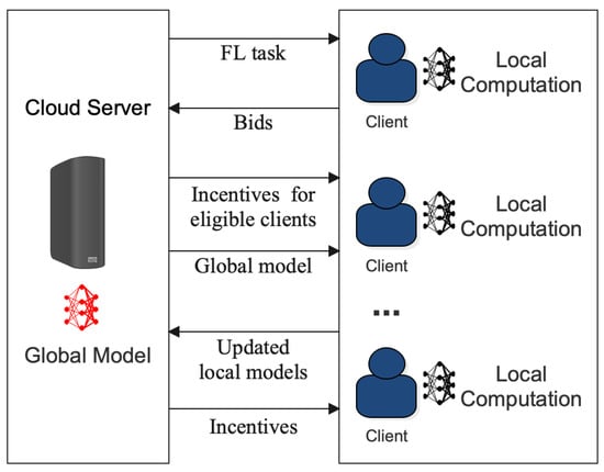 Different types of incentive mechanisms can be used to encourage participation in FL. Some of the commonly used incentive mechanisms are explained below:

• Monetary incentives: Monetary incentives involve rewarding the clients with a monetary value for their contributions. This approach can effectively motivate the clients to contribute actively to the system ^[94][171]. However, it may not be practical in all situations, as it requires a budget to support the incentive program.
• Reputation-based incentives: Reputation-based incentives are based on the principle of recognition and reputation. The clients who contribute actively and provide high-quality updates to the system can be recognized and rewarded with a higher reputation score ^[95][172]. This approach can effectively motivate the clients to contribute to the system actively.
• Token-based incentives: Token-based incentives involve rewarding the clients with tokens that can be used to access additional features or services ^[96][173]. This approach can effectively motivate the clients to contribute actively to the system and help build a vibrant ecosystem around the FL system.

The choice of incentive mechanism depends on the system’s specific requirements and the clients’ nature. In general, the incentive mechanism should be designed to align the clients’ interests with the system’s goals. One of the critical factors to consider while designing an incentive mechanism for communication costs in FL is the clients’ privacy concerns ^[97][174].

5.4. Adaptive Aggregation

Adaptive aggregation is a method for reducing communication costs in FL systems. In FL, data are typically distributed across multiple devices, and the goal is to train a machine learning model using this decentralized data. To accomplish this, the data are typically aggregated on a central server, which can be computationally expensive and lead to high communication costs ^[98][99][178,179]. Adaptive aggregation seeks to mitigate these costs by dynamically adjusting the amount of aggregated data based on the communication bandwidth of the selected client ^[100][180]. The basic idea behind adaptive aggregation is to adjust the amount of data sent to the central server based on the available bandwidth of the devices. This means that devices with slow or limited connectivity can send fewer data, while faster or more reliable connectivity can send more data. Adaptive aggregation can reduce the overall communication costs of FL systems by adapting the amount of data sent ^[101][181].

6. Optimization Techniques

6.1. Compression Schemes

Compression schemes involve techniques that reduce the models’ size and gradients exchanged between the client devices and the central server. This is necessary because the communication costs of exchanging large models and gradients can be prohibitively high, especially when client devices have limited bandwidth or computing resources ^[102][103][30,188].

6.1.1. Quantization

Quantization is a popular technique that involves representing the model or gradient values using a smaller number of bits than their original precision ^[104][189]. For instance, instead of representing a model parameter using a 32 bit floating-point number, it can be represented using an 8 bit integer. This reduces the number of bits that need to be transmitted and can significantly reduce communication costs.

6.1.2. Sparsification

Sparsification is another commonly used compression technique that involves setting a large proportion of the model or gradient values to zero ^[105][190]. This reduces the number of non-zero values that need to be transmitted, which can result in significant communication savings. Sparsification can be achieved using techniques such as thresholding, random pruning, and structured pruning.

• Thresholding is a popular technique for sparsification that involves setting all model or gradient values below a certain threshold to zero ^[106][191]. This reduces the number of non-zero values that need to be transmitted, which can result in significant communication savings. The threshold can be set using various techniques, such as absolute thresholding, percentage thresholding, and dynamic thresholding. Absolute thresholding involves setting a fixed threshold for all values, whereas percentage thresholding involves setting a threshold based on the percentage of non-zero values. Dynamic thresholding involves adjusting the threshold based on the distribution of the model or gradient values ^[107][192].
• Random pruning is another sparsification technique that randomly sets some model or gradient values to zero ^[108][123]. This reduces the number of non-zero values that need to be transmitted and can result in significant communication savings. Random pruning can be achieved using techniques like Bernoulli sampling and stochastic rounding ^[109][193]. Bernoulli sampling involves setting each value to zero with a certain probability, whereas stochastic rounding involves rounding each value to zero with a certain probability.
• Structured pruning is a sparsification technique that sets entire rows, columns, or blocks of the model or gradient matrices to zero ^[110][194]. This reduces the number of non-zero values that need to be transmitted and can result in significant communication savings. Structured pruning can be achieved using various techniques like channel, filter, and tensor pruning.

6.1.3. Low-Rank Factorization

Low-rank factorization is a compression technique that involves representing the model or gradient matrices using a low-rank approximation ^[111][112][196,197]. This reduces the number of parameters that need to be transmitted and can significantly reduce communication costs. Low-rank factorization can be achieved using techniques such as Singular Value Decomposition (SVD) ^[113][198] and Principal Component Analysis (PCA) ^[114][199]. However, low-rank factorization can also introduce some errors in the model or gradient values, which can affect the quality of the learning process.

6.2. Structured Updates

Structured updates are another important optimization technique in FL that can reduce communication costs by transmitting only the updates to the changed model parameters. This is necessary because, in many FL scenarios, only a small proportion of the client devices update their local models in each round of communication, and transmitting the entire model can be wasteful ^[11][115][11,202]. Structured updates involve identifying the parts of the model that have been updated and transmitting only those parts to the central server. Various techniques can be used to achieve structured updates, such as gradient sparsification and weight differencing [8].