CondenseNeXtV2 | Encyclopedia MDPI

CondenseNeXtV2: Comparison

Please note this is a comparison between Version 3 by Catherine Yang and Version 2 by Catherine Yang.

CondenseNeXtV2 is inspired by and is an improvement over CondenseNeXt convolutional neural network (CNN). The primary goal of CondenseNeXtV2 CNN is to further improve performance and top-1 accuracy of the network.

CondenseNeXt
convolutional neural network
computer vision

1. Convolutional Layers

CondenseNeXtV2 utilizes depthwise separable convolution which enhances the efficiency of the network without having to transform an image over and over again, resulting in reduction in number of FLOPs and an increase in computational efficiency in comparison to standard group convolutions. Depthwise separable convolution is comprised of two distinct layers:

Depthwise convolution: This layer acts like a filtering layer which applies depthwise convolution to a single input channel. Consider an image of size $X$ × $X$ × $I$ given as an input with $I$ number of input channels of the input image with kernels ( $K$ ) of size $K$ × $K$ × 1, the output of this depthwise convolution operation will be $Y$ × $Y$ × $I$ resulting in reduction of spatial dimensions whilst preserving $I$ number of channels (depth) of the input image. The cost of computation for this operation can be mathematically represented as follows:
Pointwise convolution: This layer acts like a combining layer which performs linear combination of all outputs generated by the previous layer since the depth of input image from previous operation hasn’t changed. Pointwise convolution operation is performed using a 1 × 1 kernel i.e., $1$ ×

A depthwise separable convolution splits a kernel into two distinct layers for filtering and combining operations resulting in an improvement in overall computational efficiency. Figure 1 provides a 3D visual representation of depthwise separable convolution operation where a single image is transformed only once and then this transformed image is elongated to over 128 channels. This allows the CNN to extract information at different levels for coarseness. For example, consider a green channel from the RGB channel being processed. Depthwise separable convolution will extract different shades of color green from this channel.

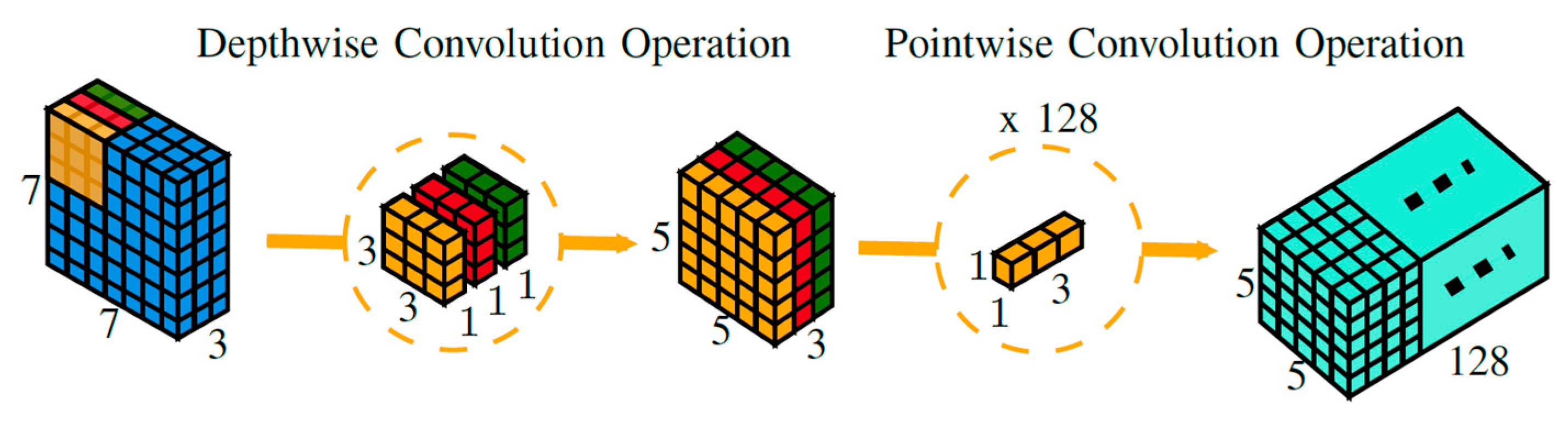
Figure 1. A 3D visual representation of depthwise separable convolution for a given example.

2. Model Compression

2.1. Network Pruning

Network pruning is one of the effective ways to reduce computational costs by discarding redundant and insignificant weights that do not affect the overall performance of a DNN. Figure 2 provides a visual comparison of weight matrices for different pruning approaches as follows:

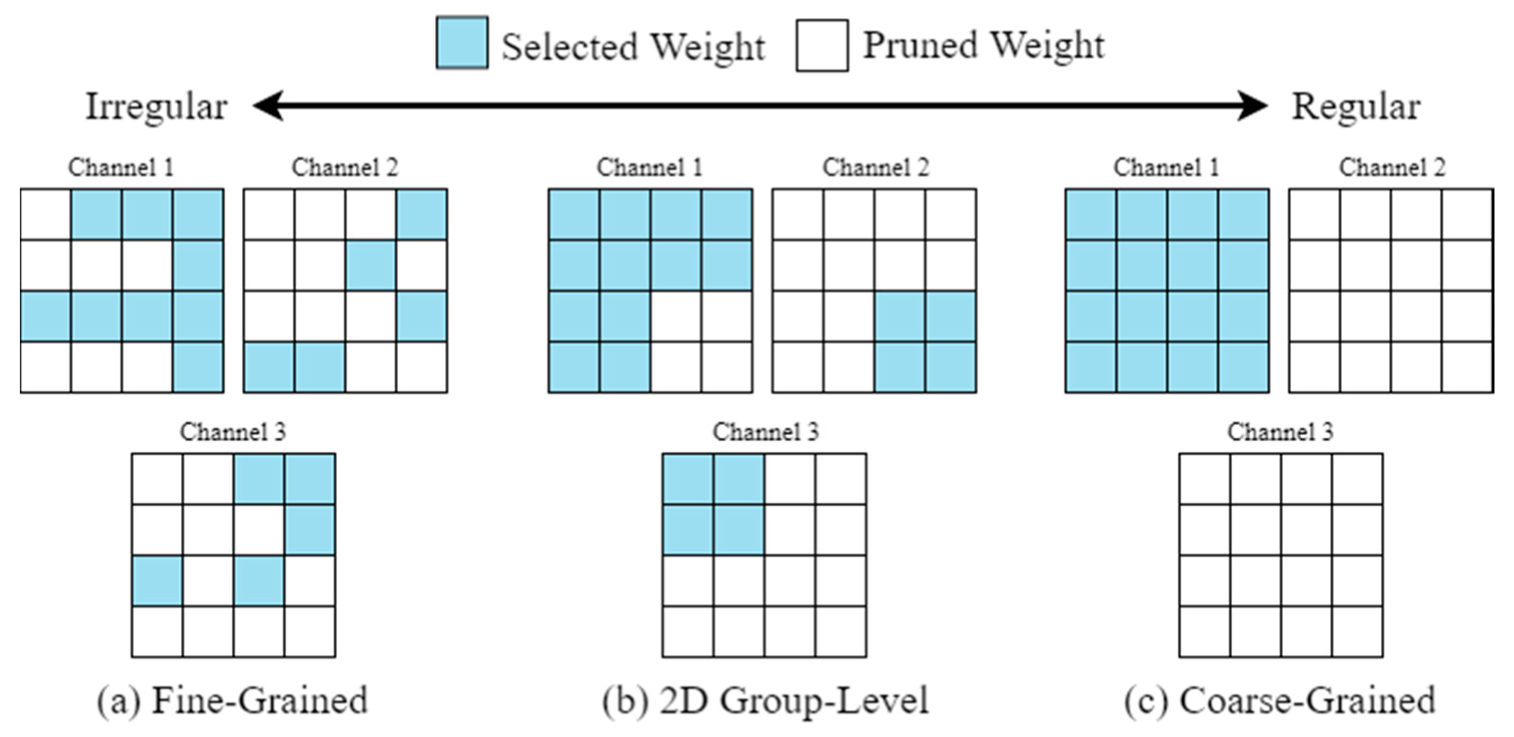
Figure 2. Comparison of different pruning methods.

Fine-grained pruning: using this approach, redundant weights that will have minimum influence on accuracy will be pruned. However, this approach results in irregular structures.

$1$
$1$ × $K$ resulting in the size of the output image to be $Y$ × $Y$ × $K$ . The cost of computation for this operation can be mathematically represented as follows:

Coarse-grained pruning: using this approach, an entire filter which will have minimal influence on overall accuracy is discarded. This approach results in regular structures. However, if the network is highly compressed, there may be significant loss in the overall accuracy of the DNN.
2D group-level pruning: this approach maintains a balance of both, benefits and trade-offs of fine-grained and coarse-grained pruning.

Pointwise convolution: This layer acts like a combining layer which performs linear combination of all outputs generated by the previous layer since the depth of input image from previous operation hasn’t changed. Pointwise convolution operation is performed using a 1 × 1 kernel i.e., $1$ × $1$ × $K$ resulting in the size of the output image to be $Y$ × $Y$ × $K$ . The cost of computation for this operation can be mathematically represented as follows:

CondenseNeXtV2 CNN utilizes 2D Group-Level pruning to discard insignificant filters which is complemented by

L_{1}

-Normalization ^[1] to facilitate the group-level pruning process.

2.2. Class-Balanced Focal Loss (CFL) Function

Pruning networks in order to discard insignificant and redundant elements of the network can still have an overall harsh effect caused due to imbalanced weights. Therefore, in order to mitigate any such issues, CondenseNeXtV2 CNN incorporates a weighting factor inversely proportional to the total number of samples, called Class-balanced Focal Loss (CFL) Function ^[2]. This approach can be mathematically represented as follows:

2.3. Cardinality

A new dimension, called Cardinality, is added to the existing spatial dimensions of the CondenseNeXtV2 network to prevent loss in overall accuracy during the pruning process, denoted by

D

. Increasing cardinality rate is a more effective way to obtain a boost in accuracy instead of going wider or deeper within the network. Cardinality can be mathematically represented as follows:

3. Data Augmentation

Data augmentation is a popular technique to increase the amount of data and its diversity by modifying already existing data and adding newly created data to existing data in order to improve the accuracy of modern image classifiers. CondenseNeXtV2 utilizes AutoAugment data augmentation technique to pre-process target dataset to determine the best augmentation policy with the help of Reinforcement Learning (RL). AutoAugment primarily consists of following two parts:

Search Space: Each policy consists of five sub-policies and each sub-policy consists of two operations that can be performed on an image in a sequential order. Furthermore, each image transformation operation consists of two distinct parameters as follows:

o

The probability of applying the image transformation operation to an image.

o

The magnitude with which the image transformation operation should be applied to an image.

There are a total of 16 image transformation operations. 14 operations belong to the PIL (Python Imaging Library) which provides the python interpreter with image editing capabilities such as rotating, solarizing, color inverting, etc. and the remaining two operations are Cutout ^[3] and SamplePairing ^[4]. Table 6 in the ‘Supplementary materials’ section of ^[5] provides a comprehensive list of all 16 image transformation operations along with default range of magnitudes.

Search Algorithm: AutoAugment utilizes a controller RNN, a one-layer LSTM ^[6] containing 100 hidden units and 2 × 5B softmax predictions, to determine the best augmentation policy. It examines the generalization ability of a policy by performing child model (a neural network being trained during the search process) experiments on a subset of the corresponding dataset. Upon completion of these experiments, a reward signal is sent to the controller to update validation accuracy using a popular policy gradient method called Proximal Policy Optimization algorithm (PPO) ^[7] with a learning rate of 0.00035 and an entropy penalty with a weight of 0.00001. The controller RNN provides a decision in terms of a softmax function which is then fed into the controller’s next stage as an input, thus allowing it to determine magnitude and probability of the image transformation operation.

At the end of this search process, sub-policies from top five best policies are merged into one best augmentation policy with 25 sub-policies for the target dataset.

4. Activation Function

An activation function in a neural network plays a crucial role in determining the output of a node by limiting the output’s amplitude. These functions are also known as transfer functions. Activation functions help the neural network learn complex patterns of the input data more efficiently whilst requiring fewer number of neurons.

CondenseNeXtV2 CNN utilizes ReLU6 activation functions along with batch normalization before each layer. ReLU6 activation function cap units at 6 which helps the neural network learn sparse features quickly in addition to preventing gradients to increase infinitely as seen in Figure 3. ReLU6 activation function can be mathematically defined as follows:

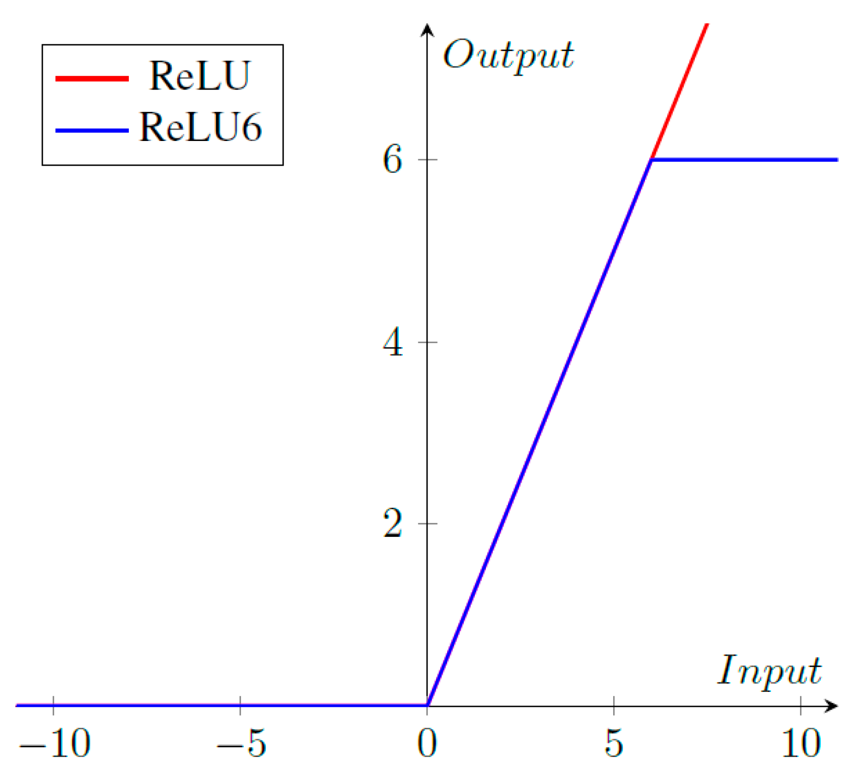
Figure 3. ReLU vs. ReLU6 activation functions.

References

Wu, S.; Li, G.; Deng, L.; Liu, L.; Wu, D.; Xie, Y.; Shi, L. L1-Norm Batch Normalization for Efficient Training of Deep Neural Networks. IEEE Trans. Neural Netw. Learn. Syst. 2019, 30, 2043–2051.
Cui, Y.; Jia, M.; Lin, T.Y.; Song, Y.; Belongie, S. Class-balanced loss based on effective number of samples. In Proceedings of the IEEE Computer Society Conference on Computer Vision and Pattern Recognition, Long Beach, CA, USA, 16–20 June 2019; pp. 9268–9277.
DeVries, T.; Taylor, G.W. Improved Regularization of Convolutional Neural Networks with Cutout. arXiv 2017, arXiv:1708.04552.
Inoue, H. Data Augmentation by Pairing Samples for Images Classification. arXiv 2018, arXiv:1801.02929.
Cubuk, E.D.; Zoph, B.; Mane, D.; Vasudevan, V.; Le, Q.V. AutoAugment: Learning Augmentation Policies from Data. Cvpr 2019, 2018, 113–123.
Hochreiter, S.; Schmidhuber, J. Long Short-Term Memory. Neural Comput. 1997, 9, 1735–1780.
Schulman, J.; Wolski, F.; Dhariwal, P.; Radford, A.; Openai, O.K. Proximal Policy Optimization Algorithms. arXiv 2017, arXiv:1707.06347.