Your browser does not fully support modern features. Please upgrade for a smoother experience.
Please note this is a comparison between Version 2 by Sirius Huang and Version 1 by Lenka Lackóová.
Remote sensing (RS) has revolutionized field data collection processes and provided timely and spatially consistent acquisition of data on the terrestrial landscape properties. The study of wind erosion involves a range of research techniques, such as laboratory and field measurements, modelling, and the use of remote sensing (RS) technologies.
- advanced remote sensing
- wind erosion
- wind erosion parameters
- wind erosion modelling
1. Introduction
Wind erosion is a natural soil degradation process [1], often accelerated by human activity [2]. The erosion events caused by wind lead to the depletion of fine particles such as clay and silt [3] and organic matter [4], which can result in decreased soil productivity and degradation of the soil’s hydrothermal properties [5]. Wind erosion (WE) predominantly occurs in regions characterized by low precipitation and high evaporation rates, which cover roughly one-third of the global land area and 12% of Europe [6]. Climate change has intensified WE in semi-arid areas by 3.2% from 1980 to 2019 [7]. The United Nations (UN) global soil resources report highlights that a significant proportion of the world’s soil is in suboptimal conditions [8]. Soil erosion, loss of soil carbon, and nutrient imbalance pose significant threats to soil functions.
The process of WE has three phases: (1) initiation of the movement of the soil particles (detachment or deflation), (2) the transportation of the soil particles (suspension, saltation, and surface creep), and (3) the deposition [9,10][9][10]. Several models have been developed to simulate the WE [11,12][11][12] and estimate the erosion intensity and effectiveness of erosion control strategies [13]. Empirical models are based on observed data and their statistical relationship with analyzed predictors. This approach is simpler, criticized for employing unrealistic assumptions, ignoring heterogeneity of inputs and nonlinear relationships between input parameters [14]. Most empirical models compute soil loss and do not simulate transportation or deposition [11]. Physical models, or process-based models, are based on understanding of the whole process of aeolian transport [15]. The distinction between the models is not always clear, and both approaches could be integrated into one model [2]. Some of the main challenges in aeolian transport modeling have been as identified the fidelity of process representation, up-scaling the presence of heterogeneity, spatial data availability, and large-scale parameter estimation [15].
The management of WE presents a formidable challenge because it involves intricate interplay due to complex interactions among driving forces, pressures, and ecosystem states [16]. Due to the intricate nature of the process, it remains challenging to oversee and measure soil WE on a larger scale [17]. The study of WE involves a range of research techniques, such as laboratory and field measurements, modelling, and the use of remote sensing (RS) technologies. While methods such as wind tunnel testing and direct terrain measurements are commonly employed, they are often constrained by time and environmental factors, and may not fully capture the complex and dynamic spatial and temporal aspects of WE. However, the accuracy of these methods is still being improved [11,18][11][18]. In the last two decades, RS [19] and computer technology have made significant progress, with increased technological potential to obtain more relevant data on WE [17]. RS methods are faster than ground methods, can cover large areas, and facilitate repeated monitoring of erosion events or factors affecting the erosion [18,20,21,22][18][20][21][22]. The employment of RS technology provides the opportunity to efficiently evaluate soil quality at different scales, with the added benefits of speed and affordability. Nevertheless, the variation in the spectral response of soils at different depths and the disparities in the spatial, spectral, and temporal resolutions of various sensors could necessitate extensive data processing and intricate models [23]. Satellite imagery allows for the quick and timely recording of the presence and intensity of erosion processes, the prediction of their impact on the topography, soils, agricultural land, and landscape systems, and approval of a set of measures to reduce the negative effects on the natural surroundings [24]. The European Space Agency’s (ESA) release of the Sentinel 2 sensor, which boasts an average spatial resolution of 10 m and a 5-day revisiting cycle, has made it one of the most widely accessible and practical sources of remote sensing data for soil erosion mapping and modeling, second only to the Landsat series [21]. The new RS systems, including drones and LiDAR, produce the data in higher spatial, temporal, and spectral resolution [18,25][18][25]. Additionally, the increasing computer power enables the large-scale application of some detailed approaches used in local scales. Incorporating RS data into WE modeling is anticipated to enhance the accuracy and decrease the level of ambiguity or imprecision present in the model [25,26][25][26].
2. Remote Sensors and Indicators Used in Wind Erosion Modelling
Recent soil survey data, such as the LUCAS topsoil and RS data, have made large-scale soil erosion modeling more feasible. LUCAS Soil, which is an extensive and recurring topsoil survey conducted every three years across the European Union, is an example of such data [30][27]. The development of dynamic indexes and proxies for soil coverage will be facilitated by the increased availability of surveyed data and the utilization of RS data (MODIS, Landsat) and Copernicus products [31][28]. Landsat, with its collection of images dating back to the Landsat Multispectral Scanner (MSS) to the Landsat Operational Land Imager (OLI) and Thermal Infrared Sensor (TIRS) is home to the oldest archive of imagery from various sensors. With a spatial resolution of 30 m, it continues to be one of the most utilized satellite images in WE modeling, as shown in Figure 31. Additionally, the Shuttle Radar Topography Mission (SRTM) data, derived from synthetic aperture radar (SAR) imagery, remain a critical source of data for erosion assessment. Other sensors, such as ASTER, Sentinel, and SPOT, among others, offer lower or medium spatial resolution.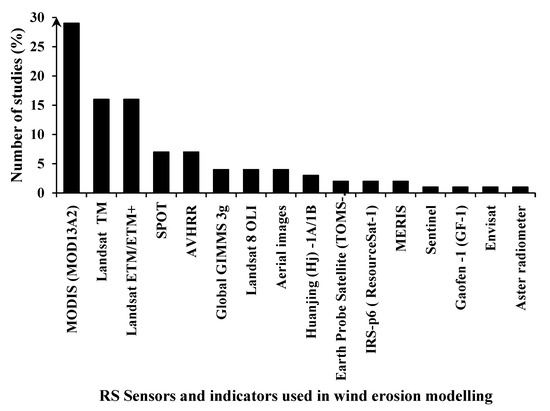
Figure 31. The percentage of global studies that employed various RS sensors and indicators for estimating WE parameters. (Note: this Figure was generated from the GASEMT database).
3. Wind Erosion Factors and RS
3.1. Soil Erodibility
Current State and Research Gaps
Erodibility, a crucial factor for predicting WE [33,34,35][30][31][32], refers to a soil’s susceptibility to erosion under specific meteorological conditions, or the efficiency of soil erosion on a surface given certain meteorological forcing. The interaction of fine soil particles (silt, clay, and sand) and organic carbon typically determines erodibility and is associated with factors such as soil structure, organic content, surface roughness, and soil texture [36][33]. However, measuring erodibility can be challenging due to these multiple factors. The influence of soil surface conditions based on soil type is often overlooked as a source of variation in characterizing soil surface erodibility and in using RS for soil assessment [37][34]. The computation of soil erodibility has been approached differently in various studies [38][35]. Ref. [39][36] calculated the wind erodibility of European soils by using a multiple regression equation based on soil texture and chemical properties, while Ref. [40][37] used soil organic carbon and soil particle size distribution to calculate erodibility in Inner Mongolia, China. However, soil erodibility equations typically require specific physical soil properties that may not be widely available. In the United States, the wind erodibility index (WEI) is available through the USDA Web Soil Survey geographic database [41][38]. Conducting long-term erosion plot studies is necessary to obtain direct measurements of soil erodibility. Most of the earlier studies [42,43,44,45][39][40][41][42] have been limited only to experimental study areas. Ref. [46][43] analyzed the soil erodibility of soil moisture, gravel cover, and surface roughness in combination with Landsat8 data to evaluate the direct impact on soil erodibility. Close-range photogrammetry was used to generate a gravel percentage map and the ASTER digital topographic model was used to analyze surface roughness. Ref. [47][44] highlighted the potential of directional and multi-angular soil reflectance to enhance the knowledge of erodibility and to detect and quantify soil erosion. In addition, the authors suggested that utilizing ground-based radiometers, as well as current and upcoming versions of angular sensors mounted on aerial and satellite platforms, and multi-angular spectral reflectance holds promise for remotely assessing and computing soil surface characteristics, thereby offering a comprehensive framework. Bi-directional soil spectral reflectance models [48,49][45][46] have the potential to establish a framework for integrating the analysis of soil surface erodibility and potentially measuring WE. Ref. [50][47] employed Landsat MSS and AVIRIS imagery to illustrate the movement of sand from deserted agricultural areas.Future Directions
Remote sensing is a valuable and economical means of obtaining data for mapping and modeling soil properties, soil resources, and their temporal and spatial variations [47,51,52,53,54][44][48][49][50][51]. Utilizing Visible, Near Infrared, and Shortwave Infrared sensors, it is possible to calibrate site-specific datasets that depict the correlation between spatiotemporal and quantitative variations in soil information across extensive regions [53][50]. Ref. [55][52] estimated soil erodibility by the support vector regression method on Landsat-8 images with relative percent deviation equals 2.01. The presence of vegetation, crop residues, or clouds can hinder the accuracy of soil property predictions, which is why extracting spectral information solely from bare soil pixels may yield successful results [56][53]. Ref. [57][54] stated that a single satellite image provides only 0.5% of valid bare soil pixels, which is inadequate for soil mapping. To address this, new methods of bare soil detection, especially from Landsat and Sentinel images, are being employed. Ref. [58][55] used the MID-Infrared profile of four images to identify bare soil pixels and established a correlation between the amount of clay content and these pixels to generate a soil clay content map. Refs. [59,60][56][57] used a fusion technique, which increased the exposed soil coverage from 36% (single image) to 75%. Meanwhile, Ref. [61][58] utilized a five-year compilation of Landsat TM imagery and the Barest Soil Composite Image (BSCI) technique to achieve 90% in soil mapping. In a similar attempt, Ref. [62][59] integrated the reflectance and spectral parameters obtained from Sentinel-2 images with a wider range of spectral and non-spectral covariates to forecast topsoil clay content. Ref. [63][60] also proved that multi-temporal images performed better in predicting soil properties, then single-date images. The Soil Composite Mapping Processor (SCMaP) was devised by [64][61] to surmount the obstacle of insufficient soil exposure and to map soil properties in Germany. Further research advancement and improvement is expected as high signal-to-noise ratio spectrometers on space-borne imagery become available, along with the PRISMA, such as EnMAP [65][62], HISUI [66][63], SHALOM [67][64], HySpex [68][65], and the Sentinel-10/CHIME [69][66].3.2. Soil Moisture
Current State and Research Gaps
The presence of soil moisture is a significant contributor to the cohesion of soil particles and acts as a mitigating factor for wind erosion [16]. Soil erodibility reaches its peak when the soil is completely dehydrated. However, as the soil moisture content increases beyond this limit, there is a noticeable reduction in erodibility. Erodibility rapidly increases with the soil moisture content [70][67]. Precisely monitoring and estimating the spatial and temporal changes in soil moisture is of great significance [71][68]. Estimating soil moisture becomes more challenging in regions with dense vegetation or snow cover, as well as areas with intricate topography [72][69]. Soil moisture content in correlation with the number of erosive days could predict some mitigation effect for some areas [39][36]. The production of dust is connected to the annual diversity in plant cover resulting from the variation in soil moisture [50][47]. Traditional techniques of restoration and reclamation necessitate surface disturbance and rely on adequate moisture to avoid erosion, making them vulnerable to significant erosion risk in the absence of wet conditions [16]. Several machine learning algorithms have been utilized for extracting water bodies and shorelines from remote sensing images, including neural networks, convolutional neural networks, artificial neural networks, support vector machines, naive Bayes, random forest, gradient boosted machine, recursive partitioning and regression trees, and constraint energy minimizations [73][70]. Individual spot measurements do not capture high spatial and temporal variability [74,75][71][72] and therefore are not suitable for regional and global research [71,76][68][73].3.3. Surface Roughness
Current State and Research Gaps
Surface roughness refers to the way surfaces are expressed in terms of topography, including features on horizontal and vertical scales ranging from millimeters to a few hundred meters [29][74]. Precise understanding of surface roughness and its influence on wind speed is crucial for various fields, including climate modeling, wind power meteorology, agriculture, and erosion hazard assessment [89][75]. Nearly flat surfaces with loose sand-sized particles, lacking any shelter or cover objects, are particularly sensitive to WE [90][76]. Surface roughness can be considered a direct input parameter or indirectly estimated through soil moisture or vegetation biomass in WE modeling [91,92][77][78]. It can be utilized as a WE predictor by determining the potential for soil particle retention, emission, and saltation [93][79]. However, the measurement accuracy of surface roughness is constrained by the measurement method, instruments used, and data pre-processing [94][80]. Surface roughness can be measured using contact or non-contact methods. Contact methods include the grid plate and profiler methods, while non-contact methods include laser profiler, stereophotography, pencil-beam radiometer, and LiDAR [95,96][81][82]. Achieving the required measurement accuracy is challenging due to limitations such as large spatial sampling intervals, short sampling segments, temporal variability, and inconvenient operation. However, TLS as a non-contact device [97][83] can furnish spatial data of high resolution (in mm), depicting surface alterations over time [98][84]. Other surface properties can be derived from the strength of the reflected signal. The best machine learning approaches for surface roughness estimation consist of both classical machine learning algorithms such as random forest, neural network and support vector machine and artificial neural network (ANN), as well as deep learning algorithms including multilayer perceptron (MLP) and deep belief network (DBN) [99][85].3.4. Vegetation Cover
Current State and Research Gaps
Vegetation reduces WE as follows: 1. safeguards the soil from erosive influences by enveloping a portion of its surface; 2. diminishes the velocity of the wind near the ground; 3. traps the soil particles [107][86]. Vegetation represents mainly standing live and dead biomass (e.g., crops in various development stages) and standing or flat litter (e.g., crop residues). The impact of vegetation on soil erodibility is contingent upon various factors such as the extent of vegetation cover, height, and spatial distribution or arrangement within a landscape [108][87]. The establishment of vegetation cover and development of windbreaks are the most common erosion control measures [18]. The impact of vegetation on WE in drylands has been primarily studied through wind tunnel experiments, windbreak studies, and field trials [107][86]. The degree of vegetation’s influence on WE is determined by the amount, height, and distribution of vegetation in the landscape. During different seasons, the state of vegetation cover undergoes changes, which in turn affects its ability to mitigate wind erosion. The impact of seasonality on vegetation cover relates to the growth and development stages of crops or plant species. In some regions, vegetation cover may decrease during dry seasons or winter, leading to reduced erosion control capacity. Conversely, during the rainy seasons or periods of active growth, the vegetation cover tends to increase, providing greater protection against erosion. The extent of vegetation cover is often represented as the ratio of the surface area covered by plants [109][88]. If the vegetation cover is below 20%, it has a minimal impact on reducing wind velocity, while erosion is essentially halted if the vegetation cover exceeds 60% [110][89]. Therefore, understanding the seasonality of vegetation cover is crucial for assessing its effectiveness in erosion control throughout the year. The review focusing on erosion monitoring [111][90] identified Landsat, SPOT, and MODIS data as the most-used RS systems for state-based monitoring of ground cover and identified the products most suitable for erosion monitoring [112,113,114][91][92][93]. For the WE modelling, the information about vegetation cover, its annual dynamics, and crop residues are important. Vegetation cover for the European scale model [115][94] was estimated from the Leaf Area Index derived from ENVISAT/MERIS satellite images. For the European WE model (WEELS), the Land Use data were gathered from existing maps, farmers files, agricultural statistics, or the land use dataset was estimated through modeling techniques in case of unavailability [36][33]. In [116][95]’s study on the East Africa region, the vegetation cover fraction was obtained from GCLS SPOT/PROBA-V images at a resolution of 1 km. For the East Africa region, Ref. [116][95] used a fraction of vegetation cover derived from GCLS SPOT/PROBA-V images at 1 km resolution. For the regional studies, the data from MODIS with a resolution of 250 m or 1 km [117,118,119][96][97][98] or Landsat with a resolution of 30 m [120,121][99][100] are often used. The pre-processed data products from Copernicus Global Land Services are also used [122][101]. For the historical analyses of the vegetation cover development, the MODIS data were combined with 8 km spatial resolution AVHRR [40,123,124][37][102][103] or the Landsat data were used [125][104]. Vegetation cover is often derived from the Normalised Difference Vegetation Index [126][105] using a dimidiate pixel model [127][106] or a specific regression model is developed [122][101]. From the range of vegetation indexes the Average Maximum Modified Soil Adjusted Vegetation Index was also used [120,128][99][107]. A classical RS classification approach was also used for the vegetation cover estimation [125][104]. In small experimental areas, the vegetation cover could be visually mapped in the field [129][108], using the line transect method [130][109] or a pin-type profile meter [131][110]. The impact of vegetation cover can be disregarded when examining the potential for WE [132][111], or in the case where the erosion events are expected at a time when there is no vegetation cover in the field [133][112]. Support Vector Regression and Random Forests are two popular classic machine learning algorithms, and have been widely used in regression and classification of vegetation-related studies [134][113].3.5. Living Wind Barriers
Current State and Research Gaps
The windbreaks have various functions in landscapes. Beside the soil protection against wind and water erosion, they positively affect the microclimate, plant productivity [150[114][115],151], soil properties [152[116][117][118],153,154], biodiversity, and also serve other purposes such as protecting buildings, offering thermal comfort to livestock, reducing snow and sand accumulation, and mitigating wind impacts on the transportation infrastructure [155][119]. Therefore, the effect of windbreaks is evaluated from different perspectives [156,157][120][121]. The WE model incorporates three aspects of wind barriers: (1) wind barriers’ height; (2) optical porosity; (3) wind barriers’ width. The wind barriers’ height affects the shelter length [158][122]. For the erosion modelling purpose, the height is measured by altimeter [159][123] or from vertical images of the windbreak [132][111], or is estimated from the average height of windbreak types [160][124]. Ref. [161][125] estimated the average tree height of windbreaks from first principal component of GF-1 Multi-Spectral high resolution satellite image. Porosity refers to the proportion of open space to the occupied space of tree stems, branches, twigs, and leaves. It impacts the degree of wind speed reduction and shelter effect of windbreaks [162][126]. Since measuring aerodynamic porosity is challenging, optical porosity is used as an alternative. Optical porosity is calculated as the ratio of white pixels to the total pixels in digitized black and white pictures taken at a distance of 30 m from the windbreak [163][127]. These images are processed using software such as ImageTool 3.0 or GIMP 2.10.34 [132,159,164,165][111][123][128][129]. In RS-based windbreak studies, it is common to assume an approximate shape for the simulated trees. However, this approach often results in notable discrepancies between the simulated and actual results. Ref. [166][130] employed TLS to obtain parameters used in a quantitative structural model (AdQSM) to reconstruct the tree structure and restore the wind field environment using the computational fluid dynamics software PHOENICS-2022. The findings suggest that TLS can effectively retrieve windbreak parameters and quantify porosity, thereby substantially improving the credibility of windbreak impact investigations in windbreak forests. The wind barriers’ width is related to barrier porosity [161[125][129],165], but also has a specific effect on wind velocity [167][131]. Using 10 m SPOT5 images is applicable for windbreaks’ width measurement; however, errors may arise when the windbreak is presented on both sides of the road, in the case of sparse or young windbreaks [168][132]. Aerial images were analyzed using object-oriented image analysis to map the windbreaks [169[133][134][135],170,171], but also for the automatic extraction of wind barriers’ width [172][136]. The wind barriers are neglected in regional scale models [17,35[17][32][36][95][101][137],39,116,122,173], because such a dataset does not exist for large areas. In most of the local studies, the effect of wind barriers is modelled in the direction of prevailing winds [159,165][123][129] or as a Euclidean distance from the nearest windbreak [161][125]. The most innovative methodology is to calculate the wind reduction for all wind directions and to weight them according to the average occurrence of erosive winds [132][111]. A unique method is to estimate the shelter area from lateral cover and shadows derived from the multitemporal MODIS albedo images [147][138].3.6. Wind Erosion Mapping
Current State and Research Gaps
RS approach is used more often for deriving the inputs for WE models, than for mapping the eroded areas. The sole effect of WE is hard to recognize from RS images; therefore, the compound effect with water erosion [187][139], tillage erosion [188][140], or land degradation in general [20,21][20][21] is mapped. Monitoring of agricultural soil degradation by RS was reviewed by the authors of [21] and they identified two RS approaches for mapping the WE: (1) mapping direct indicators such as surface lowering or changes in surface roughness; and (2) mapping indirect indicators based on WE relationship with changes in vegetation cover. One illustration of the initial approach involves utilizing radar remote sensing to delineate the patterns of wind-induced land deterioration in the northeast Patagonian region [189][141]. A second approach could be illustrated by a study that used ASTER images to obtain a WE risk map for Inner Mongolia from the basis of the land use classes, and vegetation height [190][142]. Ref. [187][139] summarized the contribution of RS to mapping land depletion in Latin America and Caribbean. The most-used WE indicators were sand dunes, however various surface erosion features such as wind streaks, desert pavements, paleo–aeolian sand features, sand encroachments, blowouts, and changes in vegetation cover were used as well. Machine learning models commonly employed for wind erosion mapping in various environmental research areas encompass decision tree models, linear equation models, particle swarm optimization-adaptive network-based fuzzy inference system, genetic algorithms, support vector regression, artificial neural networks, hybrid models, random forest, Wang and Mendel’s method, partial least square regression, principal component regression, Cubist, Bayesian additive regression trees, radial basis function, extreme gradient boosting, and regression tree analysis [188][140].References
- Sterk, G.; Riksen, M.; Goossens, D. Dryland Degradation by wind erosion and its control. Ann. Arid Zone 2001, 41, 351–367.
- Shao, Y. Physics and Modelling of Wind Erosion; Springer Science & Business Media: New York, NY, USA, 2008.
- Li, J.; Okin, G.S.; Alvarez, L.; Epstein, H. Quantitative effects of vegetation cover on wind erosion and soil nutrient loss in a desert grassland of southern New Mexico, USA. Biogeochemistry 2007, 85, 317–332.
- Yan, H.; Wang, S.; Wang, C.; Zhang, G.; Patel, N. Losses of soil organic carbon under wind erosion in China. Glob. Chang. Biol. 2005, 11, 828–840.
- Peng, F.; Xue, X.; You, Q.; Huang, C.; Dong, S.; Liao, J.; Duan, H.; Tsunekawa, A.; Wang, T. Changes of soil properties regulate the soil organic carbon loss with grassland degradation on the Qinghai-Tibet Plateau. Ecol. Indic. 2018, 93, 572–580.
- Borrelli, P.; Panagos, P.; Montanarella, L. New insights into the geography and modelling of wind erosion in the European agricultural land. Application of a spatially explicit indicator of land susceptibility to wind erosion. Sustainability 2015, 7, 8823–8836.
- Ma, X.; Zhao, C.; Zhu, J. Aggravated risk of soil erosion with global warming—A global meta-analysis. CATENA 2021, 200, 105129.
- Food and Agriculture Organization of the United Nations—FAO; Intergovernmental Technical Panel on Soils—ITPS. Status of the World’s Soil Resources (SWSR)—Main Report; Food and Agriculture Organization of the United Nations and Intergovernmental Technical Panel on Soils: Rome, Italy, 2015; p. 650.
- Lyles, L. Erosive wind energy distributions and climatic factors for the West. J. Soil Water Conserv. 1983, 38, 106–109.
- Stallings, J.H. Mechanics of Wind Erosion; TP 98; U.S. Department of Agriculture, Soil Conservation Service; U.S. Government Publishing Office: Washington, DC, USA, 1951.
- Jarrah, M.; Mayel, S.; Tatarko, J.; Funk, R.; Kuka, K. A review of wind erosion models: Data requirements, processes, and validity. CATENA 2020, 187, 104388.
- Seo, I.W.; Lim, C.S.; Yang, J.E.; Lee, S.P.; Lee, D.S.; Jung, H.G.; Lee, K.S.; Chung, D.Y. An overview of applicability of WEQ, RWEQ, and WEPS models for prediction of wind erosion in lands. Korean J. Agric. Sci. 2020, 47, 381–394.
- Blanco-Canqui, H.; Lal, R. Principles of Soil Conservation and Management; Springer Science & Business Media: Berlin/Heidelberg, Germany, 2008.
- Merritt, W.; Letcher, R.; Jakeman, A. A review of erosion and sediment transport models. Environ. Model. Softw. 2003, 18, 761–799.
- Raupach, M.R.; Lu, H. Representation of land-surface processes in Aeolian transport models. Environ. Model. Softw. 2004, 19, 93–112.
- Middleton, N.; Kang, U. Sand and Dust Storms: Impact Mitigation. Sustainability 2017, 9, 1053.
- Wang, W.; Samat, A.; Ge, Y.; Ma, L.; Tuheti, A.; Zou, S.; Abuduwaili, J. Quantitative soil wind erosion potential mapping for Central Asia using the Google Earth Engine Platform. Remote Sens. 2020, 12, 3430.
- Dwivedi, R.S. Geospatial Technologies for Land Degradation Assessment and Management, 1st ed.; CRC Press: Boca Raton, FL, USA, 2018.
- Funk, R. Assessment and measurement of Wind Erosion. In Novel Methods for Monitoring and Managing Land and Water Resources in Siberia; Springer Water Book Series; Springer: Cham, Switzerland, 2015; pp. 425–449.
- Shoshany, M.; Goldshleger, N.; Chudnovsky, A. Monitoring of agricultural soil degradation by remote-sensing methods: A Review. Int. J. Remote Sens. 2013, 34, 6152–6181.
- Sepuru, T.K.; Dube, T. An appraisal on the progress of remote sensing applications in soil erosion mapping and monitoring. Remote Sens. Appl. Soc. Environ. 2018, 9, 1–9.
- Senanayake, S.; Pradhan, B.; Huete, A.; Brennan, J. A review on assessing and mapping soil erosion hazard using geo-informatics technology for farming system management. Remote Sens. 2020, 12, 4063.
- De Paul Obade, V.; Lal, R. Assessing land cover and soil quality by remote sensing and Geographical Information Systems (GIS). CATENA 2013, 104, 77–92.
- Lukyanchuk, K.A.; Kovalchuk, I.P.; Pidkova, O.M. Application of a remote sensing in monitoring of Erosion Processes. Geoinform. Theor. Appl. Asp. 2020, 2020, 1–5.
- Zhang, J.; Guo, W.; Zhou, B.; Okin, G.S. Drone-based remote sensing for research on wind erosion in drylands: Possible applications. Remote Sens. 2021, 13, 283.
- Jiang, C.; Li, D.; Wang, D.; Zhang, L. Quantification and assessment of changes in ecosystem service in the three-river headwaters region, China as a result of climate variability and land cover change. Ecol. Indic. 2016, 66, 199–211.
- Orgiazzi, A.; Ballabio, C.; Panagos, P.; Jones, A.; Fernández-Ugalde, O. Lucas soil, the largest expandable soil dataset for Europe: A Review. Eur. J. Soil Sci. 2017, 69, 140–153.
- Panagos, P.; Katsoyiannis, A. Soil erosion modelling: The new challenges as the result of policy developments in Europe. Environ. Res. 2019, 172, 470–474.
- Phinzi, K.; Ngetar, N.S. The assessment of water-borne erosion at catchment level using GIS-based Rusle and Remote Sensing: A Review. Int. Soil Water Conserv. Res. 2019, 7, 27–46.
- Bryan, R.B. The development, use and efficiency of indices of soil erodibility. Geoderma 1968, 2, 5–26.
- Geeves, G.W.; Leys, J.F.; McTainsh, G.H. Soil erodibility. In Soils: Their Properties and Management; Charman, P.E.V., Murphy, B.W., Eds.; Oxford University Press: New York, NY, USA, 2000; pp. 205–220.
- Borrelli, P.; Ballabio, C.; Panagos, P.; Montanarella, L. Wind erosion susceptibility of European soils. Geoderma 2014, 232–234, 471–478.
- Cohen, M.J.; Shepherd, K.D.; Walsh, M.G. Empirical reformulation of the universal soil loss equation for erosion risk assessment in a tropical watershed. Geoderma 2005, 124, 235–252.
- Chappell, A.; Zobeck, T.M.; Brunner, G. Using on-nadir spectral reflectance to detect soil surface changes induced by simulated rainfall and wind tunnel abrasion. Earth Surf. Process. Landf. 2005, 30, 489–511.
- Webb, N.P.; Strong, C.L. Soil erodibility dynamics and its representation for wind erosion and dust emission models. Aeolian Res. 2011, 3, 165–179.
- Borrelli, P.; Panagos, P.; Ballabio, C.; Lugato, E.; Weynants, M.; Montanarella, L. Towards a Pan-European assessment of land susceptibility to wind erosion. Land Degrad. Dev. 2014, 27, 1093–1105.
- Zhou, Y.; Guo, B.; Wang, S.; Tao, H. An estimation method of soil wind erosion in Inner Mongolia of China based on Geographic Information System and remote sensing. J. Arid. Land 2015, 7, 304–317.
- Richardson, C.; Sadler, T. Evaluating wind erosion sensitivity for landfill sites in New Mexico using fuzzy analytical hierarchy process (FAHP). Am. J. Civ. Eng. 2022, 10, 1–12.
- Odeh, I.O.; McBratney, A.B. Using AVHRR images for spatial prediction of clay content in the Lower Namoi Valley of Eastern Australia. Geoderma 2000, 97, 237–254.
- Sullivan, D.G.; Shaw, J.N.; Rickman, D. IKONOS imagery to estimate surface soil property variability in two Alabama physiographies. Soil Sci. Soc. Am. J. 2005, 69, 1789–1798.
- Selige, T.; Böhner, J.; Schmidhalter, U. High resolution topsoil mapping using hyperspectral image and field data in multivariate regression modeling procedures. Geoderma 2006, 136, 235–244.
- Gomez, C.; Lagacherie, P.; Coulouma, G. Regional predictions of eight common soil properties and their spatial structures from hyperspectral Vis–Nir Data. Geoderma 2012, 189–190, 176–185.
- Rayegani, B.; Barati, S.; Goshtasb, H.; Gachpaz, S.; Ramezani, J.; Sarkheil, H. Sand and dust storm sources identification: A remote sensing approach. Ecol. Indic. 2020, 112, 106099.
- Chappell, A.; Zobeck, T.M.; Brunner, G. Using bi-directional soil spectral reflectance to model soil surface changes induced by rainfall and wind-tunnel abrasion. Remote Sens. Environ. 2006, 102, 328–343.
- Pinty, B.; Verstraete, M.M.; Dickinson, R.E. A physical model for predicting bidirectional reflectances over bare soil. Remote Sens. Environ. 1989, 27, 273–288.
- Jacquemoud, S.; Baret, F.; Hanocq, J. Modeling spectral and bidirectional soil reflectance. Remote Sens. Environ. 1992, 41, 123–132.
- Okin, G.S.; Murray, B.; Schlesinger, W.H. Degradation of sandy arid shrubland environments: Observations, process modelling, and management implications. J. Arid. Environ. 2001, 47, 123–144.
- Agbu, P.A.; Fehrenbacher, D.J.; Jansen, I.J. Soil property relationships with Spot Satellite Digital Data in East Central Illinois. Soil Sci. Soc. Am. J. 1990, 54, 807–812.
- Ben-Dor, E.; Chabrillat, S.; Demattê, J.; Taylor, G.; Hill, J.; Whiting, M.; Sommer, S. Using imaging spectroscopy to study soil properties. Remote Sens. Environ. 2009, 113, S38–S55.
- Mulder, V.; De Bruin, S.; Schaepman, M.; Mayr, T. The use of remote sensing in soil and terrain mapping—A review. Geoderma 2011, 162, 1–19.
- Wulf, H.; Mulder, T.; Schaepman, M.; Keller, A.; Jörg, P.C. Remote Sensing of Soils; University of Zurich, Remote Sensing Laboratories: Zurich, Switzerland, 2015.
- Chakherlou, S.; Jafarzadeh, A.A.; Ahmadi, A.; Feizizadeh, B.; Shahbazi, F.; Darvishi Boloorani, A.; Mirzaei, S. Soil wind erodibility and erosion estimation using landsat satellite imagery and multiple-criteria decision analysis in Urmia Lake Region, Iran. Arid Land Res. Manag. 2022, 37, 71–91.
- Castaldi, F.; Chabrillat, S.; Don, A.; Van Wesemael, B. Soil Organic Carbon Mapping using lucas topsoil database and sentinel-2 data: An approach to reduce soil moisture and crop residue effects. Remote Sens. 2019, 11, 2121.
- Demattê, J.A.; Fongaro, C.T.; Rizzo, R.; Safanelli, J.L. Geospatial Soil Sensing System (GEOS3): A powerful data mining procedure to retrieve soil spectral reflectance from satellite images. Remote Sens. Environ. 2018, 212, 161–175.
- Shabou, M.; Mougenot, B.; Chabaane, Z.; Walter, C.; Boulet, G.; Aissa, N.; Zribi, M. Soil Clay content mapping using a time series of Landsat TM data in semi-arid lands. Remote Sens. 2015, 7, 6059–6078.
- Demattê, J.A.; Alves, M.R.; Terra, F.D.; Bosquilia, R.W.; Fongaro, C.T.; Barros, P.P. Is it possible to classify topsoil texture using a sensor located 800 km away from the surface? Rev. Bras. Ciência Solo 2016, 40, e0150335.
- Demattê, J.A.M.; Safanelli, J.L.; Paiva, A.F.D.S.; Souza, A.B.; Dos Santos, N.V.; Nascimento, C.M.; De Mello, D.C.; Bellinaso, H.; Neto, L.G.; Amorim, M.T.A.; et al. Bare Earth’s surface spectra as a proxy for Soil Resource Monitoring. Sci. Rep. 2020, 10, 4461.
- Diek, S.; Fornallaz, F.; Schaepman, M.E.; De Jong, R. Barest pixel composite for agricultural areas using Landsat Time Series. Remote Sens. 2017, 9, 1245.
- Loiseau, T.; Chen, S.; Mulder, V.L.; Dobarco, M.R.; Richer-De-Forges, A.C.; Lehmann, S.; Bourennane, H.; Saby, N.P.A.; Martin, M.P.; Vaudour, E.; et al. Satellite data integration for soil clay content modelling at a national scale. Int. J. Appl. Earth Obs. Geoinf. 2019, 82, 101905.
- Silvero, N.E.; Demattê, J.A.; Vieira, J.D.S.; Mello, F.A.D.O.; Amorim, M.T.A.; Poppiel, R.R.; Mendes, W.D.S.; Bonfatti, B.R. Soil property maps with satellite images at multiple scales and its impact on management and classification. Geoderma 2021, 397, 115089.
- Rogge, D.; Bauer, A.; Zeidler, J.; Mueller, A.; Esch, T.; Heiden, U. Building an exposed soil composite processor (SCMAP) for mapping spatial and temporal characteristics of soils with landsat imagery (1984–2014). Remote Sens. Environ. 2018, 205, 1–17.
- Guanter, L.; Kaufmann, H.; Segl, K.; Foerster, S.; Rogass, C.; Chabrillat, S.; Kuester, T.; Hollstein, A.; Rossner, G.; Chlebek, C.; et al. The ENMAP Spaceborne Imaging Spectroscopy Mission for Earth Observation. Remote Sens. 2015, 7, 8830–8857.
- Matsunaga, T.; Iwasaki, A.; Tsuchida, S.; Tanii, J.; Kashimura, O.; Nakamura, R.; Yamamoto, H.; Tachikawa, T.; Rokugawa, S. Current Status of Hyperspectral Imager Suite (HISUI) Jadeite. In Proceedings of the 2013 IEEE International Geoscience and Remote Sensing Symposium—IGARSS, Melbourne, Australia, 21–26 July 2013.
- Varacalli, G.N.; Kafri, A.; Tidhar, G.A.; Chen, M.; Feingersh, T.; Sagi, E.; Cisbani, A.; Baroni, M.; Labate, D.; Nadler, R.; et al. SHALOM—Space-borne hyperspectral applicative land and ocean mission. In Proceedings of the 5th Workshop on Hyperspectral Image and Signal Processing: Evolution in Remote Sensing (WHISPERS), Gainesville, FL, USA, 26–28 June 2013; pp. 1–4.
- Ward, K.J.; Chabrillat, S.; Brell, M.; Castaldi, F.; Spengler, D.; Foerster, S. Mapping Soil Organic Carbon for airborne and simulated enmap imagery using the Lucas Soil Database and a local PLSR. Remote Sens. 2020, 12, 3451.
- Nieke, J.; Rast, M. Status: Copernicus Hyperspectral Imaging Mission for the Environment (CHIME). In Proceedings of the IGARSS 2019—2019 IEEE International Geoscience and Remote Sensing Symposium, Yokohama, Japan, 28 July–2 August 2019.
- Chepil, W.S. Soil Conditions That Influence Wind Erosion; Technical Bulletins 157333; United States Department of Agriculture, Economic Research Service: Washington, DC, USA, 1958.
- Wang, L.; Qu, J.J. Satellite remote sensing applications for Surface Soil Moisture Monitoring: A Review. Front. Earth Sci. China 2009, 3, 237–247.
- Ahmed, A.; Nichols, S.; Zhang, Y. Review and evaluation of remote sensing methods for soil-moisture estimation. J. Photonics Energy 2011, 2, 028001.
- Niu, L.; Kaufmann, H.; Xu, G.; Zhang, G.; Ji, C.; He, Y.; Sun, M. Triangle Water Index (TWI): An Advanced Approach for More Accurate Detection and Delineation of Water Surfaces in Sentinel-2 Data. Remote Sens. 2022, 14, 5289.
- Engman, E.T. Applications of microwave remote sensing of soil moisture for water resources and Agriculture. Remote Sens. Environ. 1991, 35, 213–226.
- Wood, E.F.; Lettenmaier, D.P.; Zartarian, V.G. A land-surface hydrology parameterization with subgrid variability for general circulation models. J. Geophys. Res. 1992, 97, 2717.
- Cheng, M.; Li, B.; Jiao, X.; Huang, X.; Fan, H.; Lin, R.; Liu, K. Using multimodal remote sensing data to estimate regional-scale soil moisture content: A case study of Beijing, China. Agric. Water Manag. 2022, 260, 107298.
- Yang, X.; Leys, J. Mapping wind erosion hazard in Australia using Modis-derived ground cover, soil moisture and climate data. IOP Conf. Ser. Earth Environ. Sci. 2014, 17, 012275.
- Petersen, R.L. A wind tunnel evaluation of methods for estimating surface roughness length at industrial facilities. Atmos. Environ. 1997, 31, 45–57.
- MacKinnon, D.J.; Clow, G.D.; Tigges, R.K.; Reynolds, R.L.; Chavez, P. Comparison of aerodynamically and model-derived roughness lengths (zo) over diverse surfaces, central Mojave Desert, California, USA. Geomorphology 2004, 63, 103–113.
- Levin, N.; Ben-Dor, E.; Kidron, G.J.; Yaakov, Y. Estimation of surface roughness (Z0) over a stabilizing coastal dune field based on vegetation and topography. Earth Surf. Process. Landf. 2008, 33, 1520–1541.
- Turner, R.; Panciera, R.; Tanase, M.A.; Lowell, K.; Hacker, J.M.; Walker, J.P. Estimation of soil surface roughness of agricultural soils using Airborne Lidar. Remote Sens. Environ. 2014, 140, 107–117.
- Moreno, R.G.; Álvarez, M.D.; Alonso, A.T.; Barrington, S.; Requejo, A.S. Tillage and soil type effects on soil surface roughness at semiarid climatic conditions. Soil Tillage Res. 2008, 98, 35–44.
- Zheng, X.; Zhao, K.; Li, X.; Li, Y.; Ren, J. Improvements in farmland surface roughness measurement by employing a new laser scanner. Soil Tillage Res. 2014, 143, 137–144.
- Davidson, M.; Thuy Le Toan Mattia, F.; Satalino, G.; Manninen, T.; Borgeaud, M. On the characterization of Agricultural Soil Roughness for radar remote sensing studies. IEEE Trans. Geosci. Remote Sens. 2000, 38, 630–640.
- Zribi, M.; Ciarletti, V.; Taconet, O. Validation of a rough surface model based on fractional Brownian geometry with SIRC and Erasme Radar Data over orgeval. Remote Sens. Environ. 2000, 73, 65–72.
- Buckley, S.J.; Howell, J.; Enge, H.; Kurz, T. Terrestrial Laser Scanning in geology: Data Acquisition, processing and accuracy considerations. J. Geol. Soc. 2008, 165, 625–638.
- Nield, J.M.; Bryant, R.G.; Wiggs, G.F.; King, J.; Thomas, D.S.; Eckardt, F.D.; Washington, R. The dynamism of salt crust patterns on playas. Geology 2015, 43, 31–34.
- Hu, X.; Shi, L.; Lin, L.; Magliulo, V. Improving surface roughness lengths estimation using machine learning algorithms. Agric. For. Meteorol. 2020, 287, 107956.
- Mayaud, J.; Webb, N. Vegetation in drylands: Effects on wind flow and aeolian sediment transport. Land 2017, 6, 64.
- Webb, N.P.; McGowan, H.A.; Phinn, S.R.; McTainsh, G.H. Auslem (Australian land erodibility model): A tool for identifying wind erosion hazard in Australia. Geomorphology 2006, 78, 179–200.
- Fryrear, D.W.; Bilbro, J.D.; Saleh, A.; Schomberg, H.; Stout, J.E.; Zobeck, T.M. RWEQ: Improved Wind Erosion Technology. J. Soil Water Conserv. 2000, 55, 183–189.
- Zhao, Y.; Wu, J.; He, C.; Ding, G. Linking wind erosion to ecosystem services in drylands: A landscape ecological approach. Landsc. Ecol. 2017, 32, 2399–2417.
- Leys, J.; McTainsh, G.; Strong, C.; Heidenreich, S.; Biesaga, K. DustWatch: Using community networks to improve wind erosion monitoring in Australia. Earth Surf. Process. Landf. 2008, 33, 1912–1926.
- Donohue, R.J.; Roderick, M.L.; McVicar, T.R. Deriving consistent long-term vegetation information from AVHRR reflectance data using a cover-triangle-based framework. Remote Sens. Environ. 2008, 112, 2938–2949.
- Goulevitch, B.; Danaher, T.; Walls, J. The statewide Landcover and trees study (slats) monitoring land cover change and greenhouse gas emissions in Queensland. In Proceedings of the IEEE 1999 International Geoscience and Remote Sensing Symposium, IGARSS’99 (Cat. No.99CH36293), Hamburg, Germany, 28 June–2 July 1999.
- Guerschman, J.P.; Hill, M.J.; Renzullo, L.J.; Barrett, D.J.; Marks, A.S.; Botha, E.J. Estimating fractional cover of photosynthetic vegetation, non-photosynthetic vegetation and bare soil in the Australian Tropical Savanna Region upscaling the EO-1 Hyperion and Modis sensors. Remote Sens. Environ. 2009, 113, 928–945.
- Panagos, P.; Borrelli, P.; Meusburger, K.; Alewell, C.; Lugato, E.; Montanarella, L. Estimating the soil erosion cover-management factor at the European scale. Land Use Policy 2015, 48, 38–50.
- Fenta, A.A.; Tsunekawa, A.; Haregeweyn, N.; Poesen, J.; Tsubo, M.; Borrelli, P.; Panagos, P.; Vanmaercke, M.; Broeckx, J.; Yasuda, H.; et al. Land susceptibility to water and wind erosion risks in the East Africa Region. Sci. Total Environ. 2020, 703, 135016.
- Guo, B.; Zhang, F.; Yang, G.; Sun, C.; Han, F.; Jiang, L. Improved estimation method of soil wind erosion based on remote sensing and geographic information system in the Xinjiang Uygur autonomous region, China. Geomat. Nat. Hazards Risk 2017, 8, 1752–1767.
- Guoli, G.; Jiyuan, L.; Quanqin, S.; Jun, Z. Sand-fixing function under the change of vegetation coverage in a wind erosion area in northern China. J. Resour. Ecol. 2014, 5, 105–114.
- Mezősi, G.; Blanka, V.; Bata, T.; Kovács, F.; Meyer, B. Estimation of regional differences in wind erosion sensitivity in Hungary. Nat. Hazards Earth Syst. Sci. 2015, 15, 97–107.
- Saadoud, D.; Hassani, M.; Martin Peinado, F.J.; Guettouche, M.S. Application of fuzzy logic approach for wind erosion hazard mapping in Laghouat region (Algeria) using remote sensing and GIS. Aeolian Res. 2018, 32, 24–34.
- Yue, Y.; Shi, P.; Zou, X.; Ye, X.; Zhu, A.; Wang, J. The measurement of wind erosion through field survey and remote sensing: A case study of the mu us desert, China. Nat. Hazards 2015, 76, 1497–1514.
- Baumgertel, A.; Lukić, S.; Belanović Simić, S.; Kadović, R. Identifying areas sensitive to wind erosion—A case study of the AP vojvodina (Serbia). Appl. Sci. 2019, 9, 5106.
- Chi, W.; Zhao, Y.; Kuang, W.; He, H. Impacts of anthropogenic land use/cover changes on soil wind erosion in China. Sci. Total Environ. 2019, 668, 204–215.
- Li, J.; Ma, X.; Zhang, C. Predicting the spatiotemporal variation in soil wind erosion across Central Asia in response to climate change in the 21st Century. Sci. Total Environ. 2020, 709, 136060.
- Rezaei, M.; Sameni, A.; Fallah Shamsi, S.R.; Bartholomeus, H. Remote Sensing of land use/cover changes and its effect on wind erosion potential in southern Iran. PeerJ 2016, 4, e1948.
- Huete, A.; Didan, K.; Miura, T.; Rodriguez, E.; Gao, X.; Ferreira, L. Overview of the radiometric and biophysical performance of the Modis vegetation indices. Remote Sens. Environ. 2002, 83, 195–213.
- Gutman, G.; Ignatov, A. The derivation of the green vegetation fraction from NOAA/AVHRR data for use in numerical weather prediction models. Int. J. Remote Sens. 1998, 19, 1533–1543.
- Qi, J.; Chehbouni, A.; Huete, A.; Kerr, Y.; Sorooshian, S. A modified soil adjusted vegetation index. Remote Sens. Environ. 1994, 48, 119–126.
- Panebianco, J.E.; Buschiazzo, D.E. Effect of temporal resolution of wind data on wind erosion prediction with the revised wind erosion equation (RWEQ). Cienc. Suelo 2013, 31, 189–199.
- Rakkar, M.; Blanco-Canqui, H.; Tatarko, J. Predicting soil wind erosion potential under different corn residue management scenarios in the Central Great Plains. Geoderma 2019, 353, 25–34.
- Pi, H.; Sharratt, B.; Feng, G.; Lei, J. Evaluation of two empirical wind erosion models in arid and semi-arid regions of China and the USA. Environ. Model. Softw. 2017, 91, 28–46.
- Bartus, M.; Barta, K.; Szatmári, J.; Farsang, A. Modeling wind erosion hazard control efficiency with an emphasis on shelterbelt system and plot size planning. Z. Geomorphol. 2017, 61, 123–133.
- Kozlovsky Dufková, J.; Mašíček, T.; Lackóová, L. Using of Wind Erosion Equation in GIS. Infrastruct. Ecol. Rural Areas 2019, 2, 39–51.
- Bao, Z.; Zhang, J.; Wang, G.; Guan, T.; Jin, J.; Liu, Y.; Li, M.; Ma, T. The sensitivity of vegetation cover to climate change in multiple climatic zones using machine learning algorithms. Ecol. Indic. 2021, 124, 107443.
- Cleugh, H.A. Effects of windbreaks on airflow, microclimates and crop yields. Agrofor. Syst. 1998, 41, 55–84.
- Zheng, X.; Zhu, J.; Xing, Z. Assessment of the effects of shelterbelts on crop yields at the regional scale in Northeast China. Agric. Syst. 2016, 143, 49–60.
- Chang, X.; Sun, L.; Yu, X.; Jia, G.; Liu, J.; Liu, Z.; Zhu, X.; Wang, Y. Effect of windbreaks on particle concentrations from agricultural fields under a variety of wind conditions in the farming-pastoral ecotone of Northern China. Agric. Ecosyst. Environ. 2019, 281, 16–24.
- Holden, J.; Grayson, R.; Berdeni, D.; Bird, S.; Chapman, P.; Edmondson, J.; Firbank, L.; Helgason, T.; Hodson, M.; Hunt, S.; et al. The role of hedgerows in soil functioning within agricultural landscapes. Agric. Ecosyst. Environ. 2019, 273, 1–12.
- Wiesmeier, M.; Lungu, M.; Cerbari, V.; Boincean, B.; Hübner, R.; Kögel-Knabner, I. Rebuilding soil carbon in degraded steppe soils of Eastern Europe: The importance of windbreaks and improved cropland management. Land Degrad. Dev. 2018, 29, 875–883.
- Engineering Sciences Data Unit (ESDU). Estimation of Shelter Provided by Solid and Porous Fences; ESDU Data Item 97031; Engineering Sciences Data Unit (ESDU): London, UK, 2000.
- Li, B.; Sherman, D.J. Aerodynamics and morphodynamics of Sand Fences: A Review. Aeolian Res. 2015, 17, 33–48.
- Miri, A.; Dragovich, D.; Dong, Z. Wind flow and sediment flux profiles for vegetated surfaces in a wind tunnel and field-scale windbreak. CATENA 2021, 196, 104836.
- Yukhnovskyi, V.; Polishchuk, O.; Lobchenko, G.; Khryk, V.; Levandovska, S. Aerodynamic properties of windbreaks of various designs formed by thinning in central Ukraine. Agrofor. Syst. 2020, 95, 855–865.
- Kučera, J.; Podhrázská, J.; Karásek, P.; Papaj, V. The effect of windbreak parameters on the wind erosion risk assessment in Agricultural Landscape. J. Ecol. Eng. 2020, 21, 150–156.
- Schmidt, S.; Meusburger, K.; Figueiredo, T.; Alewell, C. Modelling hot spots of soil loss by wind erosion (solowind) in Western Saxony, Germany. Land Degrad. Dev. 2016, 28, 1100–1112.
- Yang, X.; Li, F.; Fan, W.; Liu, G.; Yu, Y. Evaluating the efficiency of wind protection by windbreaks based on remote sensing and Geographic Information Systems. Agrofor. Syst. 2021, 95, 353–365.
- Loeffler, A.E.; Gordon, A.M.; Gillespie, T.J. Optical porosity and windspeed reduction by coniferous windbreaks in southern Ontario. Agrofor. Syst. 1992, 17, 119–133.
- Kenney, W. A method for estimating windbreak porosity using digitized photographic silhouettes. Agric. For. Meteorol. 1987, 39, 91–94.
- Středová, H.; Podhrázská, J.; Litschmann, T.; Středa, T.; Rožnovský, J. Aerodynamic parameters of windbreak based on its optical porosity. Contrib. Geophys. Geod. 2012, 42, 213–226.
- Vigiak, O.; Sterk, G.; Warren, A.; Hagen, L.J. Spatial modeling of wind speed around windbreaks. CATENA 2003, 52, 273–288.
- An, L.; Wang, J.; Xiong, N.; Wang, Y.; You, J.; Li, H. Assessment of permeability windbreak forests with different porosities based on laser scanning and computational fluid dynamics. Remote Sens. 2022, 14, 3331.
- Yusaiyin, M.; Tanaka, N. Effects of windbreak width in wind direction on wind velocity reduction. J. For. Res. 2009, 20, 199–204.
- Deng, R.X.; Li, Y.; Xu, X.L.; Wang, W.J.; Wei, Y.C. Remote estimation of shelterbelt width from spot5 imagery. Agrofor. Syst. 2016, 91, 161–172.
- Burke, M.; Rundquist, B.; Zheng, H. Detection of Shelterbelt density change using historic APFO and NAIP aerial imagery. Remote Sens. 2019, 11, 218.
- Ghimire, K.; Dulin, M.W.; Atchison, R.L.; Goodin, D.G.; Shawn Hutchinson, J.M. Identification of windbreaks in Kansas using object-based image analysis, GIS techniques and field survey. Agrofor. Syst. 2014, 88, 865–875.
- Wiseman, G.; Kort, J.; Walker, D. Quantification of shelterbelt characteristics using high-resolution imagery. Agric. Ecosyst. Environ. 2009, 131, 111–117.
- Yang, X.; Yu, Y.; Fan, W. A method to estimate the structural parameters of windbreaks using remote sensing. Agrofor. Syst. 2016, 91, 37–49.
- Pásztor, L.; Négyesi, G.; Laborczi, A.; Kovács, T.; László, E.; Bihari, Z. Integrated Spatial Assessment of Wind Erosion Risk in Hungary. Nat. Hazards Earth Syst. Sci. 2016, 16, 2421–2432.
- Chappell, A.; Webb, N.P.; Guerschman, J.P.; Thomas, D.T.; Mata, G.; Handcock, R.N.; Leys, J.F.; Butler, H.J. Improving ground cover monitoring for wind erosion assessment using MODIS BRDF parameters. Remote Sens. Environ. 2018, 204, 756–768.
- Metternicht, G.; Zinck, J.A.; Blanco, P.D.; Del Valle, H.F. Remote sensing of land degradation: Experiences from Latin America and the Caribbean. J. Environ. Qual. 2010, 39, 42–61.
- Žížala, D.; Juřicová, A.; Zádorová, T.; Zelenková, K.; Minařík, R. Mapping soil degradation using remote sensing data and ancillary data: South-East Moravia, Czech Republic. Eur. J. Remote Sens. 2018, 52 (Suppl. 1), 108–122.
- Del Valle, H.F.; Blanco, P.D.; Metternicht, G.I.; Zinck, J.A. Radar Remote Sensing of wind-driven land degradation processes in northeastern Patagonia. J. Environ. Qual. 2010, 39, 62–75.
- Reiche, M.; Funk, R.; Zhang, Z.; Hoffmann, C.; Reiche, J.; Wehrhan, M.; Li, Y.; Sommer, M. Application of satellite remote sensing for mapping wind erosion risk and dust emission-deposition in Inner Mongolia grassland, China. Grassl. Sci. 2012, 58, 8–19.
More