Improving Visual Defect Detection

Improving Visual Defect Detection: Comparison

Please note this is a comparison between Version 2 by Dean Liu and Version 3 by Dean Liu.

Reliable functionality in anomaly detection in thermal image datasets is crucial for defect detection of industrial products. Nevertheless, achieving reliable functionality is challenging, especially when datasets are image sequences captured during equipment runtime with a smooth transition from healthy to defective images. This causes contamination of healthy training data with defective samples. Anomaly detection methods based on autoencoders are susceptible to a slight violation of a clean training dataset and lead to challenging threshold determination for sample classification.

anomaly detection
deep learning
novelty detection
autoencoder
industrial image

1. Introduction

Anomaly detection is a machine learning problem in which datasets are heavily biased in favor of normal classes because the abnormal class is too small. Meanwhile, detecting unseen anomaly cases makes utilizing supervised methods impossible . These challenges lead researchers to lean towards methods that infer latent spaces. Autoencoders lie at the heart of these methods. They compress the input image to latent codings and subsequently reconstruct it. Anomaly scores can be calculated by studying the latent vector or reconstruction loss approaches. Using industrial thermal images, the research comprises a training autoencoder with two different loss functions—mean squared error (MSE) and structural similarity index measure (SSIM)—and finds anomalies within the test phase by applying three anomaly scores—MSE, SSIM, and kernel density estimation (KDE). Researchers use the term anomaly score denoted by A(x). A larger anomaly score, A(x), suggests that there are possible anomalies in the test image. Researchers group all approaches above, give their ideas, and report the survey results using classification measures. While autoencoders and alternative metrics have been extensively studied, researchers introduce a distinctive approach by utilizing KDE in conjunction with MSE or SSIM to effectively address the challenge of contaminated training data. In addition, researchers provide quantitative visualization of localized anomalies. The goal is to assist researchers in comprehending the basic concepts behind autoencoder-based visual anomaly detection, to design autoencoder models with high classification performance, and to localize defect areas on an image to find the actual defective part of the product.

2. Methodology

After the characteristics of the datasets and used data pipeline are introduced, the research method is discussed in detail. The approach consists of two phases. First, the proposed autoencoder models are developed and trained in the training phase. Then, in the test phase, anomaly score outputs are used for classification performance analyses.

2.1. Dataset and Pipeline

To evaluate the anomaly detection approaches, researchers used 32 × 32-sized thermal images of switchgear equipment. The images were captured using four infrared cameras monitoring low-voltage switchgear busbar cable connections . The cameras recorded a healthy baseline for a period of time; then, several faults were introduced to the switchgear. The faults were simply different loose cable connections that create notable intense hotspots on the thermal images.

Datasets are image sequences captured during equipment runtime. The cameras were pointed in the direction of the switchgear busbar and captured thermal images within approximately 4 h of the test time. After three hours of recording baseline healthy images, defects were introduced. Consequently, the temperature changes in the healthy data emerged on the images within a 20–30 min time window . Four scenarios were defined according to the type of loose connections, resulting in four different defective datasets: FaultL1K1, FaultL1K1K5, FaultL2K3, and FaultL2K6-7. In this context, “L” corresponds to the phase number, and “K” denotes the contact number on the busbar. To exemplify, FaultL1K1 is a loose connection in phase 1 of the first contact on the busbar accordingly. After labeling the healthy and defective images, a small amount of defective labeled data became available, which led researchers to the classic problem of imbalanced data in the anomaly detection problem.

Datasets are used using below pipeline in the experiments:

In the training phase, a model was trained with $X_{t r a i n}$ with its respective loss functions.
In the test phase, the anomaly score distributions for $X_{t r a i n}$ and $X_{d e f e c t - t e s t}$ were visualized and the threshold for classification was determined $T h r e s h o l d = m a x (A (X_{t r a i n}))$ .
$X_{h e a l t h y - c l a s s}$ and $X_{d e f e c t - c l a s s}$ were combined and used for supervised classification using the data labels $y_{h e a l t h y - c l a s s}$ and $y_{d e f e c t - c l a s s}$
The classification performance measures with $T h r e s h o l d = m a x (A (X_{t r a i n}))$ were calculated.
The false-positive rate and the true-positive rate for 30 thresholds were determined; a receiver operating characteristic (ROC) curve was drawn; and accordingly, the area under the curve (AUC) was calculated.
Result tables were prepared with the performance measures, ROC, and the AUC results.
A visualization of the healthy and defective samples was created, along with residual maps for quantitative analysis.

3. Results

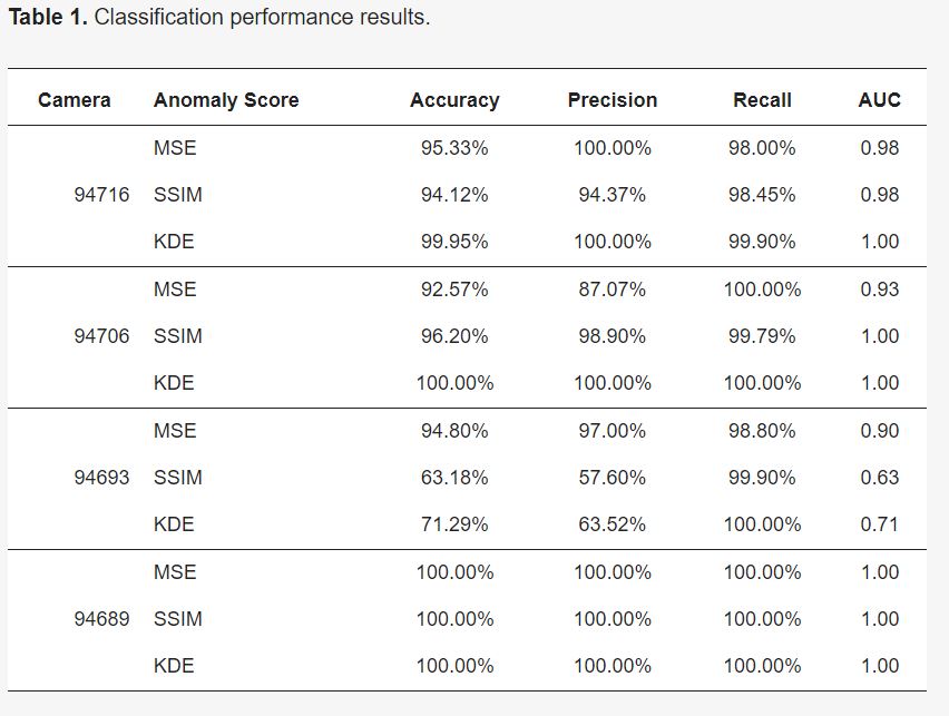
Table 1 presents the classification performance results based on the determined T on the anomaly scores generated using the autoencoder. The classification measures indicate high performances in all the datasets, except the contaminated dataset (camera 94693). This high accuracy is due to the nature of thermal images and can be reduced depending on the texture of the input images. Nevertheless, the SSIM outperforms the MSE anomaly score in all cases.

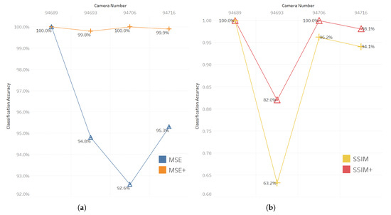
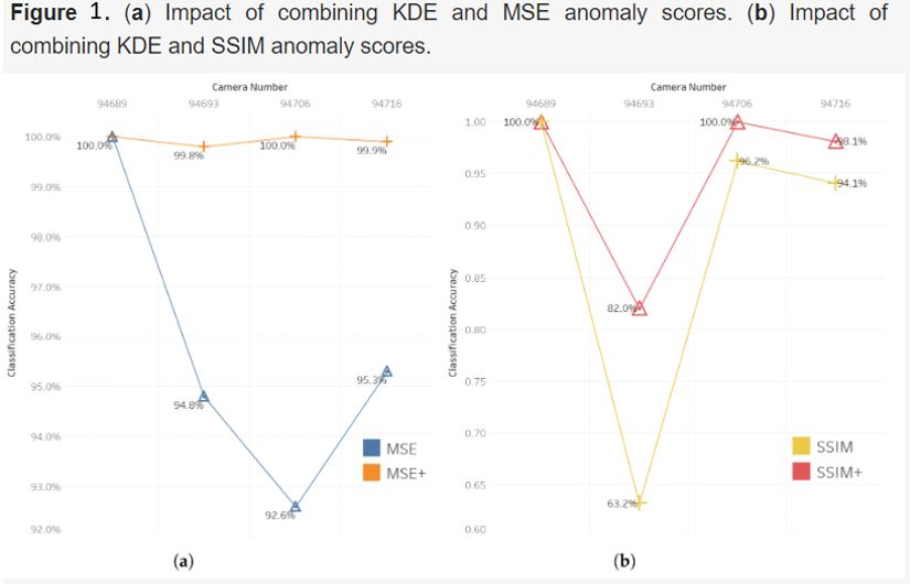
For performance improvement, researchers combined the MSE and SSIM thresholds with KDE thresholds MSE+ and SSIM+. To conduct a comparative analysis, researchers compared the results of MSE and SSIM as the baseline approaches and further evaluated the enhanced performance achieved using the MSE+ and SSIM+ thresholds. Figure 1 displays the amount of improvement in accuracy.

Figure 1. (a) Impact of combining KDE and MSE anomaly scores. (b) Impact of combining KDE and SSIM anomaly scores.