Your browser does not fully support modern features. Please upgrade for a smoother experience.
Please note this is a comparison between Version 1 by Giovanni Chiarion and Version 3 by Lindsay Dong.
Despite high-spatial-resolution imaging techniques such as functional magnetic resonance imaging (fMRI) being widely used to map this complex network of multiple interactions, electroencephalographic (EEG) recordings claim high temporal resolution and are thus perfectly suitable to describe either spatially distributed and temporally dynamic patterns of neural activation and connectivity.
- EEG
- functional connectivity
- data-driven
- signal acquisition
- pre-processing
1. Introduction
The human brain has always fascinated researchers and neuroscientists. Its complexity lies in the combined spatial- and temporal-evolving activities that different cerebral networks explicate over three-dimensional space. These networks display distinct patterns of activity in a resting state or during task execution, but also interact with each other in various spatio-temporal modalities, being connected both by anatomical tracts and by functional associations [1]. In fact, to understand the mechanisms of perception, attention, and learning; and to manage neurological and mental diseases such as epilepsy, neurodegeneration, and depression, it is necessary to map the patterns of neural activation and connectivity that are both spatially distributed and temporally dynamic.
The analysis of the complex interactions between brain regions has been shaping the research field of connectomics [2], a neuro-scientific discipline that has become more and more renowned over the last few years [3]. The effort to map the human connectome, which consists of brain networks, their structural connections, and functional interactions [2], has given life to a number of different approaches, each with its own specifications and interpretations [4][5][6][7][8][4,5,6,7,8]. Some of these methods, such as covariance structural equation modeling [9] and the dynamic causal modeling [10][11][10,11], are based on the definition of an underlying structural and functional model of brain interactions. Conversely, some others, such as Granger causality [12], transfer entropy [13], directed coherence [14][15][14,15], partial directed coherence [16][17][16,17], and the directed transfer function [18], are data-driven and based on the statistical analysis of multivariate time series. Interestingly, while non-linear model-free and linear model-based approaches are apparently unrelated, as they look at different aspects of multivariate dynamics, they become clearly connected if some assumptions, such as the Gaussianity of the joint probability distribution of the variables drawn from the data [19][20][19,20], are met. Under these assumptions, connectivity measures such as Granger causality and transfer entropy, as well as coherence [21] and mutual information rate [22][23][22,23], can be mathematically related to each other. This equivalence forms the basis for a model-based frequency-specific interpretation of inherently model-free information-theoretic measures [24]. Furthermore, emerging trends, such as the development of high-order interaction measures, are coming up in the neurosciences to respond to the need for providing more exhaustive descriptions of brain-network interactions. These measures allow one to deal with multivariate representations of complex systems [25][26][27][25,26,27], showing their potential for disentangling physiological mechanisms involving more than two units or subsystems [28]. Additionally, more sophisticated tools, such as graph theory [29][30][31][29,30,31], are widely used to depict the functional structure of the brain intended as a whole complex network where neural units are highly interconnected with each other via different direct and indirect pathways.
Mapping the complexity of these interactions requires the use of high-resolution neuroimaging techniques. A number of brain mapping modalities have been used in recent decades to investigate the human connectome in different experimental conditions and physiological states [32][33][34][32,33,34], including functional magnetic resonance imaging (fMRI) [35][36][37][38][35,36,37,38], positron emission tomography, functional near-infrared spectroscopy, and electrophysiological methods such as electroencephalography (EEG), magnetoencephalography (MEG), and electrocorticography (ECoG) [14][39][40][14,39,40]. The most known technique used so far in this context is fMRI, which allows one to map the synchronized activity of spatially localized brain networks by detecting the changes in blood oxygenation and flow that occur in response to neuronal activity [41]. However, fMRI lacks in time resolution, and therefore cannot be entrusted with detecting short-living events, which can instead be investigated by EEG, a low-cost non-invasive imaging technique allowing one to study the dynamic relations between the activity of cortical brain regions and providing different information with respect to fMRI [38]. Being exploited in a wide range of clinical and research applications [30][42][43][44][30,42,43,44], EEG has allowed researchers to identify the spatio-temporal patterns of neuronal electric activity over the scalp with huge feasibility, thanks to advances in the technologies for its acquisition, such as the development of high-density EEG systems [45][46][45,46] and their combinations with other imaging modalities, robotics or neurostimulation [47][48][49][50][47,48,49,50].
2. Brain Connectivity
Brain connectivity aims at describing the patterns of interaction within and between different brain regions. This description relies on the key concept of functional integration [51][73], which describes the coordinated activation of systems of neural ensembles distributed across different cortical areas, as opposed to functional segregation, which instead refers to the activation of specialized brain regions. Brain connectivity encompasses various modalities of interaction between brain networks, including structural connectivity (SC), functional connectivity (FC), and effective connectivity (EC). SC is perhaps the most intuitive concept of connectivity in the brain. It can be intended as a representation of the brain fiber pathways that traverse broad regions and correspond with established anatomical understanding [52][74]. As such, SC can be intended as a purely physical phenomenon. Some studies suggest that the repertoire of cortical functional configurations reflects the underlying anatomical connections, as the functional interactions between different brain areas are thought to vary according to the density and structure of the connecting pathways [52][53][54][55][56][57][58][59][74,76,77,78,79,80,81,82]. This leads to the assumption that investigating the anatomical structure of a network, i.e., how the neurons are linked together, is an important prerequisite for discovering its function, i.e., how neurons interact together, synchronizing their dynamic activity. Moreover, according to the original definition proposed in [60][75], FC does not relate to any specific direction or structure of the brain. Instead, it is purely based on the probabilities of the observed neural responses. No conclusions were made about the type of relationship between two brain regions. The only comparison is established via the presence or absence of statistical dependence. Conversely, EC was originally defined in terms of the directional influence that one neural unit exerts over another, thereby requiring the generation of a mechanistic model of the cause–effect relationships. In a nutshell, while FC was intended as an observable phenomenon quantified through measures of statistical dependencies, such as correlation and mutual information, EC was determined to explain the observed functional dependencies based on a model of directed causal influences [60][75]. In the last two decades, these concepts have been widely discussed and have evolved towards various interpretations [7][61][62][63][64][7,72,83,84,85]. EC can be assessed either from the signals directly (i.e., data-driven EC) or based on an underlying model specifying the causal pathways given anatomical and functional knowledge (i.e., EC is a combination of both SC and FC) [62][63][83,84]. The most exploited data-driven methods based on time-series analysis include adaptations of Granger causality [12][65][12,86], transfer entropy [13], partial directed coherence [16][17][16,17], and the directed transfer function [18], and are designed to identify the directed transfer of information between two brain regions. Conversely, mechanistic models of EC focus on either (i) the determination of the model parameters that align with observed correlation patterns in a given task, such as in the case of the covariance structural equation modeling [9] and dynamic causal modeling [10], or (ii) perturbational approaches to investigate the degree of causal influence between two brain regions [66][87].3. Functional Connectivity: A Classification of Data-Driven Methods
3.1. Model-Based vs. Model-Free Connectivity Estimators
AR model-based data-driven approaches typically assume linear interactions between signals. Specifically, in a linear framework, coupling is traditionally investigated by means of spectral coherence, partial coherence [16][21][67][16,21,94], correlation coefficient, and partial correlation coefficient [21]. On the other hand, different measures have been introduced for studying causal interactions, such as directed transfer function [18], directed coherence [14][15][14,15], partial directed coherence [16][17][16,17], and Granger causality [12][68][12,93]. Conversely, more general approaches, such as mutual information [60][69][75,95] and transfer entropy [13][70][13,96], can investigate non-linear dependencies between the recorded signals, starting from the definition of entropy given by Shannon [69][95] and based on the estimation of probability distributions of the observed data. Importantly, under the Gaussian assumption [19], model-free and model-based measures converge and can be inferred from the linear parametric representation of multivariate vector autoregressive (VAR) models [12][20][24][12,20,24]. Constituting the most employed metrics, linear model-based approaches are sufficient for identifying the wide range of oscillatory interactions that take place under the hypothesis of oscillatory phase coupling [6]. Linear-model-based approaches allow the frequency domain representations of multiple interactions in terms of transfer functions, partial coherence, and partial power spectrum decomposition [6][21][6,21]. This feature is extremely helpful in the study of brain signals that usually exhibit oscillatory components in well-known frequency bands, resulting from the activity of neural circuits operating as a network [71][97].3.2. Time-Domain vs. Frequency-Domain Connectivity Estimators
It is important to distinguish between time- and frequency-domain techniques, as the latter reveal connectivity mechanisms related to the brain rhythms that operate within specific frequency bands [21][39][21,39]. While approaches such as correlation, mutual information, Granger causality, and transfer entropy are linked to a time-domain representation of the data, some others, such as coherence, directed transfer function, directed coherence, and partial directed coherence, assume that the acquired data are rich in individual rhythmic components and exploit frequency-domain representations of the investigated signals. Although this can be achieved through the application of non-parametric techniques (Fourier decomposition, wavelet analysis, Hilbert transformation after band-pass filtering [72][100]), the utilization of parametric AR models has collected great popularity, allowing one to evaluate brain interactions within specific spectral bands with physiological meanings [21]. Furthermore, time-frequency analysis approaches, which simultaneously extract spectral and temporal information [73][101], have been extensively used to study changes in EEG connectivity in the time-frequency domain [74][75][76][102,103,104], and in combination with deep learning approaches for the automatic detection of schizophrenia [77][105] and K-nearest neighbor classifiers for monitoring the depth of anesthesia during surgery [78][106].4. Functional Connectivity Estimation Approaches
4.1. Time-Domain Approaches
Several time-domain approaches devoted to the study of FC have been developed throughout the years. Despite phase-synchronization measures, such as the phase locking value [79][107] and other model-free approaches [80][108] being still abundantly used in brain-connectivity analysis, linear methods are easier to use and sufficient to capture brain interactions taking place under the hypothesis that neuronal interactions are governed by oscillatory phase coupling [6]. In a linear framework, ergodicity, Gaussianity, and wide-sense stationarity (WSS) conditions are typically assumed for the acquired data, meaning that the analyzed signals are stochastic processes with Gaussian properties and preserve their statistical properties as a function of time. These assumptions are made, often implicitly, as prerequisites for the analysis, in order to assure that the linear description is exhaustive and the measures can be safely computed from a single realization of the analyzed process. Under these assumptions, the dynamic interactions between a realization of M Gaussian stochastic processes (e.g., M EEG signals recorded at different electrodes) can be studied in terms of time-lagged correlations. In the time domain, the analysis is performed via a linear parametric approach grounded on the classical vector AR (VAR) model description of a discrete-time, zero-mean, stationary multivariate stochastic Markov process, S=[X1…XM]⊺. Considering the time step n as the current time, the dynamics of S can be completely described by the VAR model [21][24][21,24]: where Sn=[X1,n…XM,n]⊺ is the vector describing the present state of S, and Spn=[S⊺n−1…S⊺n−p]⊺ describes its past states until lag p, which is the model order defining the maximum lag used to quantify interactions; Ak is the M×M coefficient matrix quantifying the time-lagged interactions within and between the M processes at lag k; and U is a M×1 vector of uncorrelated white noise with an M×M covariance matrix Σ=diag(σ211,…σ2MM). Multivariate methods based on VAR models as in (1) depend on the reliability of the fitted model, and especially the model order. While lower model orders can provide inadequate representations of the signal, orders higher than are strictly needed tend to provide overrepresentation of the oscillatory content of the process and drastically increase noise [81][109]. One should pay attention to the procedure for selecting the optimum model order, which can be set according to different criteria, such as the Akaike information criterion (AIC) [82][110] or the Bayesian information criterion (BIC) [83][111]. It should be noted that, in multichannel recordings such as with EEG data, the analysis can be multivariate, which means taking all the channels into account and fitting a full VAR model, as in (1), or it can be done by considering each channel pair separately, which means fitting a bivariate AR model (2AR) in the form of (1) with M=2: where Z=[XiXj]⊺, i,j=1,…,M (i≠j), is the bivariate process containing the investigated channel pair, with Zn=[Xi,nXj,n]⊺ and Zpn=[Z⊺n−1…Z⊺n−p]⊺ describing, respectively, the present and p past states of Z; Bk is the 2×2 coefficient matrix quantifying the time-lagged interactions within and between the two processes at lag k, and W is a 2×1 vector of uncorrelated white noises with 2×2 covariance matrix Λ. The pairwise (bivariate) approach typically provides more stable results, since it involves the fitting of fewer parameters but leads to loss of information due to the fact that only a pair of time series is taken into account [84][112]. Indeed, since there are various situations that provide significant estimates of connectivity in the absence of true interactions (e.g., cascade interactions or common inputs) [21][84][21,112], the core issue becomes whether the estimate of pairwise connectivity reflects a true direct connection between the two investigated signals or is the result of spurious dynamics between multiple time series. To answer this question, it is recommended to take into account the information from all channels when estimating the interaction terms between any pair of time series. Even if at the expense of increased model complexity resulting in a more difficult model identification process, moving from a pairwise to a multivariate approach can significantly increase the accuracy of the reconstructed connectivity patterns. This would allow distinguishing direct from indirect interactions through the use of extended formulations obtained through partialization or conditioning procedures [16][21][85][16,21,113].4.2. Frequency-Domain Approaches
To examine oscillatory neuronal interactions and identify the individual rhythmic components in the measured data, representations of connectivity in the frequency domain are often desirable. The transformation from the time domain to the frequency domain can be carried out by exploiting parametric (model-based) or non-parametric (model-free) approaches. Non-parametric signal-representation techniques are mostly based on the definition of the power spectral density (PSD) matrix of the process as the Fourier transform (FT) of Rk , on the wavelet transformation (WT) of data, or on Hilbert transformation following band-pass filtering [72][100]. In general, they bypass the issues of the ability of linear AR models to correctly interpret neurophysiological data and the selection of the optimum model order. The latter choice can be problematic, especially with brain data, because it strongly depends on the experimental task, the quality of the data and the model estimation technique [86][153]. However, the non-parametric spectral approach is somewhat less robust compared to parametric estimates, since it can be characterized by lower spectral resolution; e.g., it has been shown to be less efficient in discriminating epileptic occurrences in EEG data [87][154]. On the other hand, parametric approaches exploit the frequency-domain representation of the VAR model, in the multivariate (1) or in the bivariate (2) case, which means computing the model coefficients in the Z-domain and then evaluating the model transfer function H(ω) on the unit circle of the complex plane, where ω=2πffs is the normalized angular frequency and fs is the sampling frequency [21]. The M×M PSD matrix can then be computed using spectral factorization as where * stands for the Hermitian transpose [21]; note that Σ is replaced by Λ in the case of (2), i.e., when M=2. It is worth noting that, while the frequency-domain descriptions ubiquitously used and re viewed here are based on the VAR model representation, their key element is actually the spectral factorization theorem reported above and that approaches other than VAR models can be used to derive frequency-domain connectivity measures [88][155].4.3. Information-Domain Approaches
The statistical dependencies among electrophysiological signals can be evaluated using information theory. Concepts of mutual information, mutual information rate, and information transfer are widely used to assess the information exchanged between two interdependent systems [60][69][75,95], the dynamic interdependence between two systems per unit of time [22][23][22,23], and the dynamic information transferred to the target from the other connected systems [13][70][13,96], respectively. The main advantage of these approaches lies in the fact that they are probabilistic and can thus be stated in a fully model-free formulation. On the other hand, their practical assessment in the information domain is not straightforward because it comprises the estimation of high-dimensional probability distributions [89][180], which becomes more and more difficult as the number of network nodes increases in multichannel EEG recordings. Nevertheless, information-based metrics can also be expressed in terms of predictability improvement, such that their computation can rely on linear parametric AR models, where concepts of prediction error and conditional entropy, GC and information transfer, or TD and mutual information rate, have been linked to each other [19][20][90][91][19,20,121,181]. Indeed, it has been demonstrated that, under the hypothesis of Gaussianity, predictability improvement and information-based indexes are equivalent [19]. Based on the knowledge that stationary Gaussian processes are fully described in terms of linear regression models, a central result is that for Gaussian data, all the information measures can be computed straightforwardly from the variances of the innovation processes of full and restricted AR models [19].4.4. Other Connectivity Estimators
Brain connectivity can be estimated through a large number of analyses applied to EEG data. Multivariate time-series analysis has traditionally relied on the use of linear methods in the time and frequency domains. Nevertheless, these methods are insufficient for capturing non-linear features in signals, especially in neurophysiological data where non-linearity is a characteristic of neuronal activity [80][108]. This has driven the exploration of alternative techniques that are not limited by this constraint [80][92][108,217]. Moreover, the utilization of AR models with constant parameters, and the underlying hypotheses of Gaussianity and WSS of the data, can be key limitations when stationarity is not verified [93][218]. A number of approaches have been developed to overcome this issue, providing time-varying extensions of linear model-based connectivity estimators using adaptive AR models with time-resolved parameters, in which the AR parameters are functions of time [94][95][96][174,219,220].5. EEG Acquisition and Pre-Processing
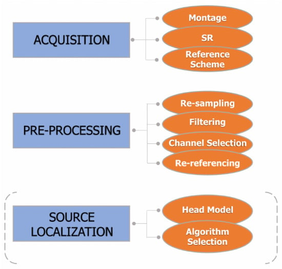
The acquisition and conditioning of the EEG signal represent two important aspects with effects on the entire subsequent processing chain. The main steps of acquisition and pre-processing are indicated in Figure 13. An example of application of the pre-processing pipeline to experimental EEG is shown in Figure 24.Figure 13. Main steps in EEG acquisition and pre-processing. In general, source localization is not mandatory, as represented by the dashed round brackets.
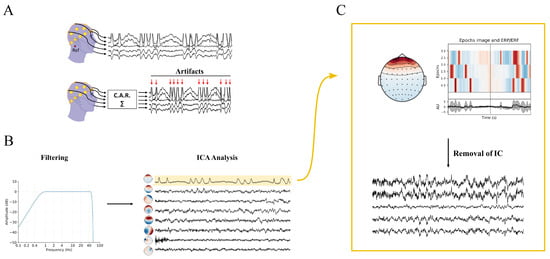
Figure 24. Schematic representation of the pre-processing pipeline applied to EEG signals acquired on the scalp (s253 recording of the subject 2 that could be found in https://eeglab.org/tutorials/10_Group_analysis/study_creation.html#description-of-the-5-subject-experiment-tutorial-data, accessed on 15 February 2023). (A) Unipolar EEG signals are acquired using a mastoid reference (Ref, in red). For clarity, only a limited number of the recorded signals, among the original 30 channels, is plotted. The average re-referencing process and the pre-processed signals are illustrated below. Notably, red arrows indicate blinking artifacts that are clearly visible. (B) The re-referenced signals are filtered using a 1–45 Hz zero-phase pass-band filter, followed by independent component analysis (ICA) to extract eight independent components (ICs), shown on the right. (C) The first IC, suspected to be an artifact, is analyzed, with a scalp-shaped heatmap assessing its localization in the frontal area and its temporary coincidence with the artifacts shown in panel (A). After removing the first IC, the cleaned signal is plotted at the bottom of the panel.
Sampling frequency, the number of electrodes, and their positioning, each have an important role in assessing connectivity; too low of a sampling frequency cannot be used to analyze high-frequency bands for the Nyquist–Shannon sampling theorem [97][296], and the electrode density defines with which accuracy and reliability further processing will be performed [40].
An EEG signal is a temporal sequence of electric potential values. The potential is measured with respect to a reference, which should be ideally the potential at a point at infinity (thus, with a stable zero value). In practice, an ideal reference cannot be found, and any specific choice will affect the evaluated connectivity [6][98][6,57]. Unfortunately, as for most of the FC analysis pipeline, there is no gold standard for referencing, and this is clearly a problem for cross-study comparability [99][297].
5.1. Resampling
Nowadays, EEG signal is usually acquired with a sampling rate (SR) equal or superior to 128 Hz, since this value is the lower base-2-power that permits one to capture most of the information content in EEG signal and a big part of the γ band. It is noticeable that high-frequency oscillations (HFOs), such as ripples (80–200 Hz) and fast ripples (200–500 Hz), will not be captured with these SRs [100][101][102][103][51,52,53,54]. Moreover, there are studies suggesting that low SRs affect correlation dimensions, and in general, non-linear metrics [104][105][55,56].5.2. Filtering and Artifact Rejection
Filtering EEG is a necessary step for the FC analysis pipeline, not only to extract the principal EEG frequency waves, but particularly to reduce the amounts of noise and artifacts present in the signal and to enhance its SNR. Research suggests the use of finite impulse response (FIR) causal filters that could be used also for real-time (RT) applications, or infinite impulse response (IIR) filters, which are less demanding in terms of filter orders but distort phase, unless they are applied with reverse filtering, thereby making the process non-causal and not applicable for RT applications. In general, if sharp cut-offs are not needed for the analysis, FIR filters are recommended, since they are always stable and easier to control [106][301]. If one is interested in investigating FC in the γ band, electrical line noise at 50 or 60 Hz could be a problem, since it is not fully removable with a low-pass filter. Notch filters are basically band-stop filters with a very narrow transition phase in the frequency domain, which in turn leads to an inevitable distortion of the signal in the time domain, such as smearing artifacts [106][301]. To avoid this problem, some alternatives have been developed. A discrete Fourier transform (DFT) filter is obtained by subtracting from the signal an estimation of the interference obtained by fitting the signal with a combination of sine and cosine with the same frequency as the interference. It avoids potential distortions of components external to the power-line frequency. It assumes that the power-line noise has constant power in the analyzed signal segment. As this hypothesis is not strictly verified in practice, it is recommended to apply the DFT technique to short data segments (1 s or less). Another proposed technique is CleanLine, a regression-based method that makes use of a sliding window and multitapers to transform data from the time domain to the frequency domain, thereby estimating the characteristics of the power line noise signal with a regression model and subtracting it from the data [107][302]. This method eliminates only the deterministic line components, which are optimal, since EEG signal is a stochastic process, but in the presence of strong non-stationary artifacts, it may fail [108][303]. It is pretty normal that EEG signals can be corrupted by many types of artifacts, defined as any undesired signal which affects the EEG signal whose origin cannot be identified in neural activity. Generators of these undesirable signals could be physiological, such as ocular artifacts (OAs such as eye blink, saccade movement, rapid eye movements), head or facial movements, muscle contraction, or cardiac activity [109][110][305,306]. Power-line noise, electrode movements (due to non-properly connected electrodes), and interference with other electrical instrumentation are non-physiological artifacts [111][307]. Artifact management is crucial in the analysis of connectivity. In fact, their presence in multiple electrodes can result in overestimation of brain connectivity, skewing the results [112][113][308,309]. The most effective way for dealing with artifacts is to apply prevention in the phase of acquisition to avoid as much as possible their presence, for example, by making acquisitions in a controlled environment, double-checking the correct positioning of electrodes, or instructing the patients to avoid blinking the eyes in certain moments of the acquisition. In fact, eye blinks are by far the most common source of artifacts in the EEG signal, especially in the frontal electrodes [114][115][312,313]. They are shown as rapid, high-amplitude waveforms present in many channels, whose magnitudes exponentially decrease from frontal to occipital electrodes. However, saccade movements produce artifacts, generating an electrooculographic signal (EOG). Acquisition of this signal, concurrently with the EEG signal, is known to be a great advantage in identifying and removing ocular artifacts, since vertical (VEOG), horizontal (HEOG), and radial (REOG) signals diffuse in different ways through the scalp [116][314]. Once the parts of the signals corrupted by the artifacts have been identified, it is still common practice to eliminate these portions, avoiding alterations on the signal that could lead to spurious connectivity. As for channel rejection, however, it is preferable to retain as much information as possible [117][316].5.3. Bad Channel Identification, Rejection, and Interpolation
It could happen that some EEG channels present a high number of artifacts (eye blink, muscular noise, etc.) or noise, due to bad electrode-scalp contact. In these cases, the rejection of these channels could be an option. However, it is necessary to check whether the deleted channels are not fundamental and the remaining channels are sufficient to carry on the analysis, considering also that deleting channels will result in an important loss of information that is likely not recovered anymore. Some authors discussed the criteria for detection of bad channels and suggested considering the proportion of bad channels with respect to the total to assess the quality of the dataset (for example, imposing a maximum of 5%) [118][329]. Identification of bad channels could be performed visually or automatically. Visual inspection requires certain experience with EEG signals to decide if a channel is actually not recoverable and needs to be rejected [119][120][330,331]. Indeed, this process is highly subjective. Automatic detection of bad channels could be performed in various ways. A channel correlation method identifies the bad channels by comparing their divergence from the Pearson correlation distribution among each pair of channels with the other couples. This method assumes high correlations between channels due to the volume-conduction effect proper of the EEG signal, which is discussed in detail in the source localization section. High standard deviation of an EEG signal can be an indicator of the presence of a great amount of noise. By setting a proper threshold, the standard deviation can be a useful index for identifying bad channels.5.4. Re-Referencing
As described in the previous section, many decisions are made during the acquisition of the signals; however, some of them are revertible. Re-referencing and down-sampling is one of them. It consists of changing the (common) reference of each EEG channel into another one by performing for each channel the addition of a fixed value (notice that it is a fixed value in space, i.e., common for all channels, but not in general constant in time). Re-reference with respect to a new reference channel can be performed by simply subtracting each channel with the new reference. In most cases, average reference (CAR) is considered to be a good choice, especially if electrodes cover a large portion of the scalp with the assumption that the algebraic sum of currents must be zero in the case of uniform density of sources [121][333]. It consists of referencing all the electrode signals with respect to a virtual reference that is the arithmetic mean of all the channel signals. Due to charge conservation, the integral of the potential over a closed surface surrounding the neural sources is zero. Obviously, the EEG channels give only a discrete sampling of a portion of that surface, so that the virtual reference can be assumed to be only approximately zero. However, it could be much better than using a single location as reference, such as an EEG channel or the mastoid (both LM and LR), which have been shown to generate larger distortion than the average reference [112][308].6. Source Connectivity Analysis
Measuring information dynamics from EEG signals on the scalp is not straightforward due to the impact of volume conduction, which can modify or obscure the patterns of information flow across EEG electrodes [122][196]. This effect is due to the electrical conductance of the skull, which serves as a support to diffuse neural activity in all the directions and for this reason is also known as field spread problem. The neural current sources are related to the Poisson equation to the electrical potential, which diffuses across the scalp and can be measured by many electrodes, also pretty far from the original source. This is the reason why interpreting scalp-level connectivity requires caution. In fact, the estimated FC between two electrodes could be reflecting the activation of a single brain region, rather than two functionally connected regions. Even though this effect can be compensated for when working with scalp EEG signals [122][123][196,197], it is often recommended to use source signal reconstruction to obtain a more accurate representation of the underlying neural network. This is because the source-based network representation is considered a more accurate approximation of the real neural network structure [124][347]. The general pipeline that source localization algorithms follow is based on this two-step loop [125][348]:-
Forward problem—definition of a set of sources and their characteristics and simulation of the signal that would be measured (i.e., the potential on the scalp) knowing the physical characteristics of the medium that makes it diffuse;
-
Inverse problem—comparison of the signal generated by the head model with the actual measured EEG and adjustment of the parameters of the source model to make them as similar as possible.