Object detection and classification have received a lot of attention in recent years due to the wide range of applications that are possible and the recent flurry of activity in computer vision research. Most applications in ITS regarding vehicle detection and classification focus a great deal of effort on traffic accident investigation, traffic flow monitoring, fleet and transport management, autonomous driving, and similar. Digital image processing techniques have been aggressively employed in recent years in vehicle shape detection, color, speed, and post estimation. Simultaneously, computational power has increased. Nowadays, computer vision-based ^[1][2][3][1,2,3] platforms are equipped with high-core processing and graphics processing units (GPUs), which detect and classify objects to pursue real-time implementations. Deep Learning (DL) and Machine Learning (ML) have exhibited vital CV research applications. Deep ConvNets have various architectures of DL on CV topics, such as image classification, object detection, object recognition, learning, vehicle tracking, object pose estimation, and others.

An image is a two-dimensional digital distribution of pixel values designated by finite numbers. The pixels are denoted on the x–y spatial coordinate axis [4]. Digital image processing is a term that describes the processing of an image or video frame, taken as input, and involving a set of phases with various parameters and experimental setups. For example, detecting a vehicle would imply that images or video frames clearly show its presence, as well as its location, in an image. Therefore, object detection can be defined as a means to locate samples of real-world objects in images. In this context, vehicle detection is closely related to vehicle classification, since it involves defining the presence and location of the vehicle in an image. However, the image is useless unless it is properly analyzed to extract useful knowledge. Hand-crafted features (namely, Histogram of Oriented Gradient (HOG) [5], Haar [6], and LBP [7]) are the most appropriate techniques to detect vehicles, but they fail to provide a general solution, and the classifiers require some modifications to fit various parameters. A shallow neural network is utilized as well for vehicle detection, though its performance has not provided the desired quality. Handling this massive amount of data necessitates the growth of an innovative method capable of performing quickly, precisely, and consistently. Advancing the efficiency of vehicle detection and classification accuracy, precision, and robustness through DL techniques, such as DCNNs, RCNNs, and DNNs, improves the robustness of schemes in detecting and classifying vehicles from images or video frames.

2. Deep Learning Techniques

Object detection, recognition, and classification in computer vision are practically helpful but technologically challenging. There are two main categories: multi-oriented object detection and classification and single object recognition. DL approaches for object detection and recognition and classification of images mainly focus on accurate object recognition (improving detection and recognition performance), speed of testing, training, computational processes, and accurate object classification (minimizing the error rate) ^[8][9][8,9]. 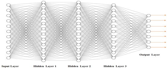Deep Learning deals with DNN architecture, where deep refers to figures of the hidden layers, and its main objective is to resolve learning problems by copying the functioning of the human brain ^[9][10][9,10]. Schemes employing DL have been developing and improving consistently, as have adjustments to the model structure. Depending on the scheme, tuning may be required or setups applied to upgrade the execution of the scheme. The designs of DCNNs often involve the following essential elements: Convolution Layer: The convolution layer is the initial layer that receives an input image and extracts the features from that data. It utilizes small input data and learns the data features by sustaining the correlation between values of pixels, which involves a filter/kernel matrix and an image matrix, and the performance of a mathematical operation to learn the features. Activation Function: Linear or non-linear activation functions are used to monitor the results of models. They can be linear or non-linear, depending on the function they monitor. Pooling Layers: These employ subsampling and spatial pooling techniques to minimize some parameters without removing the critical parameter. Various methods of pooling are employed, including average, sum, and maximum approaches. Fully Connected (FC) Layer: The final few layers are FC layers. After the final pooling or CNN layer, the output feature maps are mainly flattened (vectors) and used as input to FC layers. A Deep Nets Architecture is depicted in Figure 12.

2.1. Techniques

2.1.1. Traditional Detection Methods

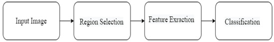
In more recent years, object recognition/detection and classification have been hot research topics in computer vision-based applications. Various objects in various environments may be challenging to detect, and, therefore, to classify and identify, due to the following factors: weather, lighting, illumination effects, size of the objects, inter-class variations, intra-class variations, and other factors. In recent studies, many extracted AI features have been employed to classify objects. The traditional feature-based object recognition and classification approaches consist of three systems (see Figure 23):

• Region selection
• Feature extraction, and
• Classification.

The most common traditional feature-based architectures in the literature for vehicle detection and recognition and classification are the Histogram of Oriented Gradient (HOG) [5], Haar [6], and LBP [7]. Haar features are calculated by adding and subtracting the sums of rectangles and the differences across an image patch. As this was highly efficient at calculating the symmetry structure in detecting vehicles [11], it was ideal for real-time detection. The Haar feature vector and the AdaBoost ^[12][13][12,13] were widely used in CV to detect objects in a variety of feature applications, including vehicle recognition [11]. HOG features are extracted in the following phases:

• Evaluating the edge and discretizing the image;
• Removing edge sharpness.

The HOG feature vector integrated with the Support Vector Machine (SVM) classifier has been widely employed to recognize object orientation, i.e., on-road vehicle detection ^[14][15][14,15]. The HOG–SVM [16] performed admirably in multi-vehicle detection tasks. In addition, a blend of HOG [5] and Haar [6] was employed for vehicle recognition, detection, and tracking [17]. Local Binary Pattern (LBP) [7] features have performed better in different applications, including texture classification, face recognition, segmentation, image retrieval, and surface crack detection. The cascade classifier (Haar–LBP–HOG feature) [18] is detects vehicles with bounding boxes. In addition to the previously mentioned features and classifiers for vehicle detection and classification problems, statistical architectures, based on horizontal and vertical edge features, were proposed for vehicle detection [19], side-view car detection [20], online vehicle detection [21], and vehicle detection in severe weather using HOG–LBP fusion [22].

2.1.2. CNN-Based Two-Step Algorithms

A two-step object detector, or the region-based approach, comprises two steps to process an image:

• Produce a series of candidate frames or extract region proposals from the scene;
• Classify and regress the generated candidate frames to improve the architecture’s detection accuracy.

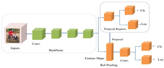
The region-based approach has the properties of high localization and performance, slower speed, and high computational cost during training. Figure 34 displays the architecture of a two-step object detector. Researchers have proposed several two-step object detector algorithms and these have been employed for vehicle detection and classification in more recent years. They are explained as follows: R-CNN: Girshick et al. [23] proposed an R-CNN or region-based ConvNet two-step object detector architecture. In ^[23][24][23,24] AlexNet was employed as the backbone model of the detector. It can increase the detection accuracy of objects over that of traditional object detection algorithms, such as HOG [5], Haar [6] and LBP [7] feature extraction. The R-CNN has four systems to accomplish the tasks. The operation of the algorithm is as follows:

• Produce categorical-independent region proposals;
• Extract a fixed-length feature vector from each region proposal;
• Compute the confidence scores to classify the object classes using class-specific support vector machines;
• Predict the bounding-box regressor for accurate bounding-box predictions, once the object class has been classified.

The authors adopted a selective search approach [25] to search for parts of the image having higher probability. Convolutional neural networks (ConvNets) were used to extract a 4096 dimensional feature vector from each proposed region. There had to be an exact match in length between the region’s proposed features and the input vectors for the FC. For the model, the authors used a fixed pixel size of 27×2727×27, regardless of the candidate region’s size or aspect ratio. When using R-CNN, the final FC is linked to the M+1+1 classification layers (hence, M represents the number of object classes and 1 represents the background) to perform the final object classification. Optimizing convolution parameters, such as IoU, is accomplished with SGD. An IoU of less than 0.50.5 is considered incorrect for a region proposal; otherwise, it is correct. In R-CNN, without sharing computation, the region proposal and classification problems are carried out independently. However, R-CNN has problems concerning computational cost and training time for classification. To solve the problem of too much time required in the training process, convolutional feature maps with high resolution can be generated at a low cost using the Fast R-CNN architecture proposed by Girshick [26]. Fast R-CNN: The Fast R-CNN [26] network takes as input an entire image and a set of object proposals. It follows the following specific steps:

• Generate a convolution feature by using various convolution and max-pooling layers on the entire image;
• Extract a fixed-length feature vector from the feature map for each object proposal of Region of Interest pooling layers;
• Feed each feature vector into a sequence of FC layers to generate softmax probability predictions over M object classes plus 1 background (M+1+1). The other layer generates four real-valued n. Fast R-CNN utilizes a streamlined training process with a fine-tuning step that jointly optimizes a softmax classifier and Bbox regressors.

Training a softmax classifier, SVMs, and regressors in separate stages accelerates the training time over the standard R-CNN architecture. The entire process architecture includes loss, the SGD optimizer, the mini-batch sampling strategy, and BP through the RoI pooling layers. However, Fast R-CNN uses a selective search approach over the convolution feature map to explore its pooling map, increasing its run time. Using a new region proposal network (RPN), Shaoqing et al. [27] proposed a faster RCNN architecture to improve the Fast RCNN network in terms of run time and detection performance in order to better estimate the object region at various aspect ratios and scales. Faster R-CNN: In terms of operation time and detection performance, the faster RCNN [27] is a more advanced variant of the RCNN. Instead of the traditional method, selective search replaces RPN’s outstanding prediction of object regions at various scales and aspect ratios. Anchors are placed at each convolutional feature location to create a variety of region proposals. The anchor box in Faster RCNN has three different aspect ratios and three different scales. It comprises four systems to achieve object detection tasks: candidate region producing, feature extraction, classification, and location fine-tuning. In the RPN architecture, the feature map is computed using a sliding window of 3×33×3, which is then output to the Bbox classification and Bbox regression layers. Each point on the feature map is traversed by the sliding window, which places z anchor boxes where they are needed. The feature map’s z anchor boxes are used to extract its elements. R-FCN: The two-step object detection architecture can be categorized into two distinct groups. One group represents classification networks like GoogleNet [28], ResNet [29], AlexNet [24], VGGNet [30]. Their computation is shared by all ROIs and an image test is conducted using one forward computation. In the second group, no computation is shared to all ROIs since it aims to classify the object regions. Dai et al. [31] proposed the R-FCN architecture of an improved version of the faster RCNN and partially eliminated the problem of position sensitivity and position variance by increasing the sharing of convolutional parameters. For the RFCN algorithm, the primary goal is the creation of “position-sensitive score maps.” If the ROI is not part of the object, it is determined by comparing it to the ROI sub-region, which consists of the corresponding parts (s×s). There is a shared convolutional layer at the end of the RFCN network’s network. An additional layer of dimensional convolution (4×s24×2) is applied to the score maps to produce class-independent Bboxes. A softmax is used to calculate the results, after averaging the s2 scores, to produce (M+1+1) dimensional vectors. A comparison study was carried out on the most widely utilized two-step object detectors on both the COCO dataset [32] and the PASCAL VOC 07 [33] dataset. In [34], experimentation showed that RCNN achieved 66%66% of the mAP on the PASCAL VOC 07 dataset [33], while Fast RCNN achieved 66%66% of the same dataset. In addition, the Fast RCNN network was nine times faster than the standard RCNN network. Wang et al. [35] conducted a comparative study on three networks, namely, fast RCNN, faster RCNN, and the RFCN, on two publicly available datasets, i.e., the COCO [32] dataset and the PASCAL VOC 07 [33] dataset. On the COCO test dataset, faster RCNN improved detection accuracy by 3.2%3.2% compared to slow RCNN. Furthermore, the tasking positions on both RFCN and the faster RCNN on both datasets were compared. The experimental results revealed that RFCN outperformed the faster RCNN with superior detection accuracy and less operational run time. 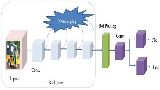There is no region proposal phase for the classification or detection of object classes in a single-step algorithm, and the prediction results are directly obtained from the image. In this algorithm, the input image is sampled at various positions uniformly, using different aspect ratios and scales, and then the CNN layer is sampled to extract features to precisely execute regression and classification. The most notable merits of the models are that they are easier to optimize, suitable for real-time applications, and faster. There is no region proposal phase for the classification or detection of object classes in a single-step algorithm, and the prediction results are directly obtained from the image. In this algorithm, the input image uses a variety of aspect ratios and scales, and the CNN layer is sampled to extract features that can be used to accurately perform regression and classification. The most notable merits of the models are that they are easier to optimize, suitable for real-time applications, and faster. Figure 45 displays the framework of the Basic Architecture of One-step Detector. Numerous single-step object detector algorithms have been utilized for various applications, such as, among others, real-time vehicle object detection, vehicle recognition, in the last couple of years. Some of the most widely employed algorithms are the following: SSD [36], RetinaNet [37], YOLO [38], YOLOv2 [39], YOLOv3 [40], YOLOv4 [41], and YOLOv5 [42]. RetinaNet Algorithm: Lin et al. [37] proposed a RetinaNet algorithm that performs the focal loss as a classification loss. It solves the class imbalance between the positive and negative samples, which minimizes the prediction accuracy. The author introduced a focal loss to minimize the weight loss by avoiding several negative samples given in the background. The algorithm utilizes the ResNet [43] model as a backbone and FPN [44] as feature extraction architecture. It consists of two processes: generating a set of region proposals via FPN and classification of each candidate. SSD Algorithm: Liu et al. [36] proposed an SSD algorithm based on a feedforward convolutional architecture that generates a fixed-size sum of bounding boxes and scores for existing object class samples, followed by an NMS stage to generate the detection process. The SSD algorithm utilizes a VGG16 [43] architecture as a backbone for feature extraction and six more convolutional layers for detection. It generates sequences of feature maps of various scales, followed by a 3×33×3 filter on each feature map to generate default Bboxes. It only detects at the top layers to get the best prediction Bbox and class label. YOLO Algorithm: The YOLO algorithm [38] is a CNN-based object detection one-step detector that was designed after two-step object detection became the faster RCNN detector. The YOLO algorithm is most applicable for real-time image detection. It has a few region proposals per image compared to the faster RCNN. It utilizes a grid size of (t×t) to split the images into grid features for image classification. Grid cells can be used to estimate Bbox bounding boxes and C class probabilities for C object classes for each box. For each box, the probability (P) and the IOU between the ground truth and the box are considered. The YOLO algorithm has 2 FC layers and 24 convolution layers. However, the algorithm has the problem of weak object localization, which affects the classification accuracy. YOLOv2 Algorithm: The YOLOv2 algorithm [39] is an improved version of the YOLO algorithm in detection precision and offers higher speed than the standard YOLO algorithm. It contains 6 consecutive tasks to efficiently perform the detection process, namely the BN, high-resolution classifier, convolution with anchor box, various aspect ratios and scales of the anchor box, fine-grained feature techniques, and multi-scale training. The training process of the YOLOv2 algorithm [39] is carried out through the SGD optimizer, which employs a mini-batch. For example, mean, mini-batch, and variance are calculated and utilized for activation purposes. Then, every mini-batch activation is normalized using the standard deviation of 1 and 0 mean. In the end, all elements in every mini-batch are sampled using an uniform distribution. This process is carried out through techniques of batch normalization (BN) [45]. It generates activation of uniform distribution to speed up its operation to obtain convergence. The YOLOv2 model uses a high-resolution classifier as a backbone to maximize the input resolution into (448×448448×448), and classification fine-tuning is implemented for image resolution with 10 epochs to improve its map by 4%. Moreover, techniques of convolution anchor box are also utilized to generate region proposals to predict the object-class score and class for each estimated Bbox, leading to an improvement of its recall by 7%7%. Furthermore, the model uses the anchor box’s size and aspect ratio prediction technique with K-means clustering. Fine-grained features for small objects and multi-scale training with image sizes of 320,352,...,608320,352,...,608 improve the detection of objects of different sizes. YOLOv3 Algorithm: The YOLOv3 Algorithm [40] is another improved version of the YOLO Algorithm. It utilizes the DarkNet53 model for feature extraction and employs a multi-label classification with overlapping patterns for the training process. It is primarily notable for object detection in complex scenes. In addition, in the YOLOv3 Algorithm, various sizes of three feature maps are utilized to predict the Bbox. The last convolution layer is used to produce a three-dimensional tensor that consists of objectness, class predictions, and Bbox. YOLOv4 Algorithm: Single-step object detection algorithms, such as the YOLOv4 Algorithm [41], combine the properties of YOLO, YOLOv2, and YOLOv3 and achieve the current optimum in terms of both accuracy and speed. The residual system receives the feature layer and outputs the higher-level feature information. Algorithms like YOLOv4 are composed of a 3 structure called the “Neck”, “Backbone”, and “Prediction” sections. The SPPNet and PANet form the neck. Features in the SPPNet are concatenated and then extremely pooled by supreme cores of various scales in the feature layer. To increase the receptive field of the architecture, the pooled result is appended and convolved 3 times and the concatenated feature layers are up-sampled after concatenating with the SPPNet and Backbone. The process was cycled to up-sample and down-sample with feature layers to achieve CSPDarkNet53 for feature fusion and compression of height and width. Then, they are layered on top of each other to create new combinations of features. The features extracted from the model can be used to make predictions according to the prediction scheme. Prediction results from a network are filtered out using the Non-maximal Suppression (NMS) [46] efficient technique. YOLOv5 Algorithm: The YOLOv5 algorithm utilizes CSPDarkNet as a backbone for the feature extraction model to extract feature information from the input data. Compared to the other variants of the YOLO algorithm, it has better capability to detect small objects, excellent detection accuracy, and is more adaptable and faster. It has 4 modules. The CSPNet architecture eliminates the gradient information duplication problem of model optimization in massive models and combines the gradient variation from the previous to the final into feature maps. Consequently, decreasing the volume of architecture FLOPS values and parameters causes the improved accuracy and speed of the model. However, it decreases the size of the architecture. The detection efficiency depends on the computation of the frame selection area to improve the model, which proposes the Fcos approach [47]. The model employs the CSPDarkNet feature extraction model to extract image features competently and utilizes Bottleneck CSP instead of a residual shortcut link to strengthen the description of the image features. The neck system is mainly employed to produce a feature pyramid. The feature pyramids can help the network find objects of different sizes, so as to find the frame object of different scales and sizes. The CNN-based object detector has been applied to many DL-based applications. Its purpose is commonly illustrated as an effective, efficient object detection, recognition, and classification application with fewer error rates. The detector has been applied to face mask recognition ^[48][49][48,49], real-time vehicle detection [50], vehicle classification [51], off-road quad-bike detection [52], pedestrian detection [53], medical image classification [54], automotive engine crack detection [55] and so on.