Radiomics in Prostate Cancer

Version	Summary	Created by	Modification	Content Size	Created at	Operation
1		Pierpaolo Purpura	+ 1458 word(s)	1458	2021-10-13 08:16:51	\|
2	Format change	Jessie Wu	Meta information modification	1458	2021-10-26 05:55:09	\| \|
3	Definition change	Peter Tang	+ 66 word(s)	1524	2021-10-26 05:58:20	\|

This entry is adapted from the peer-reviewed paper 10.3390/diagnostics11101829

Prostate cancer (PCa) is the fourth most commonly diagnosed cancer and the fifth leading cause of cancer death among men worldwide. Multiparametric MRI (mp-MRI) has gained popularity as a noninvasive imaging technique for detection of clinically significant PCa and biopsy guidance. mpMRI may overcome many of the shortcomings of the combination of PSA and TRUS alone, achieving accurate tumor detection with sensitivity of 72% and specificity of 81%. The entry analyzes the current and potential radiomics applications for prostate cancer on mpMRI.

radiomics magnetic resonance imaging prostate cancer PI-RADS Gleason score

1. Introduction

Prostate cancer (PCa) is the fourth most commonly diagnosed cancer and the fifth leading cause of cancer death among men worldwide ^[1]. PCa more frequently (80%) originates in the peripheral zone (PZ) and less commonly (15%) in the transitional zone (TZ), while the central zone (CZ) location of PCa is rare ^[2]. Albeit less common, PCa in the TZ contributes to morbidity and mortality because of confounding changes in this region due to benign prostatic hyperplasia, which is found in up to 25% of TZ cancers ^[2]. Transrectal ultrasound (TRUS) is a cost-effective and easily available imaging modality, but with limited sensitivity and specificity ranging between 40% and 50% for detection of PCa ^[3]. Multiparametric MRI (mp-MRI) has gained popularity as a noninvasive imaging technique for detection of clinically significant PCa and biopsy guidance. mpMRI may overcome many of the shortcomings of the combination of PSA and TRUS alone, achieving accurate tumor detection with sensitivity of 72% and specificity of 81% ^[4]^[5]^[6]. It is also increasingly used in patients undergoing active surveillance to monitor recurrence in patients after radiotherapy (RT) or androgen deprivation therapy (ADT). The MRI diagnostic system for prostatic lesions is known as Prostate Imaging-Reporting and Data System (PI-RADS), and the latest version (v2.1) was published in 2019 ^[5]. 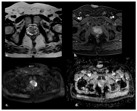This system evaluates the relative likelihood of the existence of a clinically significant prostate cancer ranging from PI-RADS 1 “clinically significant disease is highly unlikely to be present” to PI-RADS 5 “clinically significant cancer is highly likely to be present” (Figure 1). 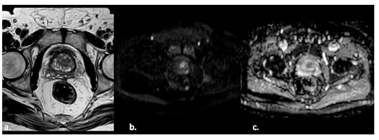The PI-RADS scoring system has high sensitivity and specificity, but still there are many lesions that are categorized as PI-RADS 3 (Figure 2) or PI-RADS 4 which means that these lesions carry a moderate to high risk of being or becoming clinically significant prostate cancer but cannot be diagnosed as such, and biopsy may be needed ^[6]^[7].

Figure 1. A 65 year old man with a PI-RADS 5 lesion in the left postero-lateral segment of the PZ of midgland, hypointense in T2-weighted images (a), with early enhancement in DCE images (b), markedly hyperintense on DWI, and hypointense on ADC images (c,d).

Figure 2. A 55-year old man with a PI-RADS 3 lesion in the left anterior segment of PZ of the midgland, moderately hypointense on T2-weighted images (a), hyperintense on DWI, and hypointense on ADC images (b,c).

In the last decade, there has been increasing interest in the quantitative analysis of imaging data. Radiomics is a relatively novel process of medicine designed to extract a large number of quantitative features from radiological images, offering a cost-effective and high-throughput approach to medical imaging data analysis using advanced mathematical algorithms, which could lead to accurate tumor detection and aid personalized cancer treatment ^[8]^[9]. Radiomics and artificial intelligence (AI) cover a wide variety of subfields and techniques. Machine learning is the subfield of AI where the algorithm is applied to a set of data and to knowledge about these data; radiologists can select and encode features that appear distinctive in the data, and the statistical techniques are used to organize the data on the basis of these features. Then, the system can learn from the training data and apply what it has learned to make a prediction (e.g., for differential diagnosis between benign or malignant lesions) ^[10]. Representation learning is a type of machine learning where the algorithm learns on its own the best features to classify the provided data. Deep learning is a type of representation learning where the algorithm learns a composition of features that reflect a hierarchy of structures in the data. This system is able to discriminate the compositional nature of images starting from simple features (intensity, edges, and textures) to elaborate more complex features such as shapes, lesions, or organs ^[11]. Thus, these systems are important in the use of radiomics in medical images because they allow collapsing clusters of big datasets into a few representative features and creating classifier models through database mining. In the last few years, deep learning has been applied to prostate cancer with promising results, although it is not yet used in the clinical routine.

The aim of this narrative review was to describe the current and potential radiomics applications for prostate cancer on mpMRI. For this purpose, we first describe the different steps of radiomic analysis, and then we provide a summary of the literature on radiomic analysis for prostate cancer.

2. Radiomics Analysis

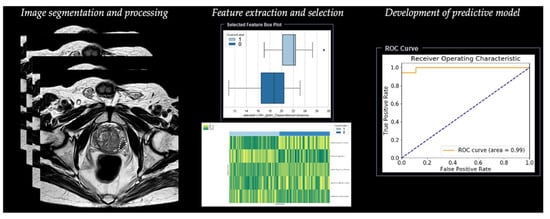
Radiomic analysis requires different steps, including segmentation, image processing, feature extraction, feature development, and development of a predictive model (Table 1) (Figure 3).

Figure 3. Workflow of radiomics for prostate cancer in a simulated study on T2-weighted images using a prototype research software Radiomics, version 1.0.9 (Siemens Healthineers, Forchheim, Germany).

Table 1. Summary of main steps for radiomics analysis.

2.1. Step 1—Segmentation

The first step is image segmentation of the region of interest (ROI) in two dimensions (2D) or of the volume of interest (VOI) in three dimensions (3D), defining the area in which radiomic features will be calculated. Image segmentation can be manual or semi-automatic (usually with manual correction), but this method is considered time-consuming and does not allow a reproducible analysis of the radiomic derived features for its intrinsic intra-observer variability ^[12]. Although there is still no universal segmentation algorithm for all image applications, the best option is automated image segmentation using atlas-based and model-based methods that avoid intra- and inter-observer variation ^[13]. These methods work well for relatively homogeneous lesions, but show the need for intensive user correction for inhomogeneous lesions, such as lesions including air voxels as one example. Haaburger et al. ^[14] proposed a neural network architecture that generates plausible segmentation after separate training using default parameters as provided in the reference implementation.

2.2. Step 2—Image Processing

The second step is image processing, and it represents the attempt to homogenize images with respect to pixel spacing, gray-level intensities, and bins of gray-level histogram. This step consists of interpolation to isotropic voxel spacing to increase reproducibility between different datasets, intensity outlier filtering (normalization) to remove pixels/voxels that fall outside of a specified range of gray-level, and discretization of image intensities, which consists of grouping the original values according to specific range intervals ^[12].

2.3. Step 3—Feature Extraction

The third step is the extraction of radiomic features. Since many different ways and formulas exist to calculate those features, adherence to the Image Biomarker Standardization Initiative (IBSI) is recommended ^[15].

Features extracted from diagnostic images are classified into two groups. The first group includes the so-called “semantic features”, represented by radiologic features commonly used to describe lesions such as shape, location, vascularity, and necrosis. The second group includes the so-called “agnostic features” that analyze lesion heterogeneity through quantitative descriptors which are subdivided in turn into first-, second-, or higher-order statistical outputs ^[8]. The distribution of individual voxel intensities without concern for a spatial relationship is described through first-order statistics. These features reduce an ROI to single values for mean, median, uniformity, or randomness (entropy), magnitude (energy), and minimum and maximum gray-level intensity. Second-order statistics, introduced in 1973 by Haralick ^[16], describe interrelationships between voxels with similar or dissimilar contrast values as “texture features”, and they can readily provide a measure of intratumoral heterogeneity; these features are based on the gray-level co-occurrence matrix (GLCM), defining the pattern of an image subregion by summarizing the appearance of voxel pairs with a specific discretized gray-level value in a specified direction, and on the gray-level run length matrix (GLRLM), summarizing the frequency of continuous voxels that have the same discretized gray-level value in a given direction ^[17]. Higher-order statistical methods impose filter grids to extract repetitive or nonrepetitive patterns ^[13].

2.4. Step 4—Feature Selection

The next step is represented by feature selection, performed to select the most useful subset of features to build statistical and machine learning models with the exclusion of nonreproducible, redundant, and nonrelevant features. Rizzo et al. ^[13] analyzed cluster analysis and principal component analysis, which are the two most commonly used unsupervised approaches. Cluster analysis creates groups of similar features (clusters), and a single feature may be selected from each cluster as representative and used in the following association analysis. Principal component analysis creates a smaller set of maximally uncorrelated variables from a large set of correlated variables, and it allows explaining the variation in the dataset with the fewest possible principal components. After the selection of the most representative features for each cluster, it is possible to develop a model fitting with these remaining features.

2.5. Step 5—Development of Predictive Model

Once features have been selected, they are used for training the predictive model. This is built with different machine learning algorithms, including support vector machine (SVM), logistic regression, random forest (RF), and decision tree (DT).

The rapid development of deep learning, such as convolutional neural network (CNN) and artificial neural network (ANN), has accelerated the pace of radiomics progress ^[18].

References

Sung, H.; Ferlay, J.; Siegel, R.L.; Laversanne, M.; Soerjomataram, I.; Jemal, A.; Bray, F. Global cancer statistics 2020: GLOBOCAN estimates of incidence and mortality worldwide for 36 cancers in 185 countries. CA Cancer J. Clin. 2021, 71, 209–249.
Ginsburg, S.B.; Ms, A.A.; Pahwa, S.; Gulani, V.; Ponsky, L.; Aronen, H.J.; Boström, P.J.; Böhm, M.; Haynes, A.; Brenner, P.; et al. Radiomic features for prostate cancer detection on MRI differ between the transition and peripheral zones: Preliminary findings from a multi-institutional study. J. Magn. Reson. Imaging 2017, 46, 184–193.
Chen, F.K.; Abreu, A.L.D.C.; Palmer, S. Utility of Ultrasound in the Diagnosis, Treatment, and Follow-up of Prostate Cancer: State of the Art. J. Nucl. Med. 2016, 57, 13S–18S.
De Rooij, M.; Hamoen, E.H.J.; Fütterer, J.J.; Barentsz, J.O.; Rovers, M.M. Accuracy of multiparametric MRI for prostate cancer detection: A meta-analysis. Am. J. Roentgenol. 2014, 202, 343–351.
Turkbey, B.; Rosenkrantz, A.B.; Haider, M.A.; Padhani, A.; Villeirs, G.; Macura, K.J.; Weinreb, J.C. Prostate Imaging Reporting and Data System Version 2.1: 2019 Update of Prostate Imaging Reporting and Data System Version 2. Eur. Urol. 2019, 76, 340–351.
Oberlin, D.T.; Casalino, D.D.; Miller, F.H.; Meeks, J.J. Dramatic increase in the utilization of multiparametric magnetic resonance imaging for detection and management of prostate cancer. Abdom. Radiol. 2017, 42, 1255–1258.
Patel, N.U.; Lind, K.E.; Garg, K.; Crawford, D.; Werahera, P.N.; Pokharel, S.S. Assessment of PI-RADS v2 categories ≥ 3 for diagnosis of clinically significant prostate cancer. Abdom. Radiol. 2019, 44, 705–712.
Gillies, R.J.; Kinahan, P.E.; Hricak, H. Radiomics: Images Are More than Pictures, They Are Data. Radiology 2016, 278, 563–577.
Vernuccio, F.; Cannella, R.; Comelli, A.; Salvaggio, G.; Lagalla, R.; Midiri, M. Radiomica e intelligenza artificiale: Nuove frontiere in medicina. Recent Prog. Med. 2020, 111, 130–135.
Erickson, B.J.; Korfiatis, P.; Akkus, Z.; Kline, T.L. Machine Learning for Medical Imaging. RadioGraphics 2017, 37, 505–515.
Chartrand, G.; Cheng, P.M.; Vorontsov, E.; Drozdzal, M.; Turcotte, S.; Pal, C.J.; Kadoury, S.; Tang, A. Deep Learning: A Primer for Radiologists. RadioGraphics 2017, 37, 2113–2131.
Van Timmeren, J.E.; Cester, D.; Tanadini-Lang, S.; Alkadhi, H.; Baessler, B. Radiomics in medical imaging-”how-to” guide and critical reflection. Insights Imaging 2020, 11, 91.
Rizzo, S.; Botta, F.; Raimondi, S.; Origgi, D.; Fanciullo, C.; Morganti, A.G.; Bellomi, M. Radiomics: The facts and the challenges of image analysis. Eur. Radiol. Exp. 2018, 2, 36.
Haarburger, C.; Müller-Franzes, G.; Weninger, L.; Kuhl, C.; Truhn, D.; Merhof, D. Radiomics feature reproducibility under inter-rater variability in segmentations of CT images. Sci. Rep. 2020, 10, 1–10.
Zwanenburg, A.; Vallières, M.; Abdalah, M.A.; Aerts, H.J.W.L.; Andrearczyk, V.; Apte, A.; Ashrafinia, S.; Bakas, S.; Beukinga, R.J.; Boellaard, R.; et al. The Image Biomarker Standardization Initiative: Standardized Quantitative Radiomics for High-Throughput Image-based Phenotyping. Radiology 2020, 295, 328–338.
Haralick, R.M.; Shanmugam, K.; Dinstein, I. Textural Features for Image Classification. IEEE Trans. Syst. Man Cybern. 1973, SMC-3, 610–621.
Galloway, M.M. Texture analysis using gray level run lengths. Comput. Graph. Image Process. 1975, 4, 172–179.
Cheng, R.; Roth, H.R.; Lay, N.; Lu, L.; Turkbey, B.; Gandler, W.; McCreedy, E.S.; Pohida, T.; Pinto, P.A.; Choyke, P.; et al. Automatic magnetic resonance prostate segmentation by deep learning with holistically nested networks. J. Med. Imaging 2017, 4, 041302.

© Text is available under the terms and conditions of the Creative Commons Attribution (CC BY) license; additional terms may apply. By using this site, you agree to the Terms and Conditions and Privacy Policy.

Upload a video for this entry

Information

Subjects: Radiology, Nuclear Medicine & Medical Imaging

Contributor MDPI registered users' name will be linked to their SciProfiles pages. To register with us, please refer to https://encyclopedia.pub/register :

Pierpaolo Purpura

View Times: 387

Update Date: 26 Oct 2021

Table of Contents

Video Upload Options

Confirm