Submitted Successfully!
To reward your contribution, here is a gift for you: A free trial for our video production service.
Thank you for your contribution! You can also upload a video entry or images related to this topic.
Version Summary Created by Modification Content Size Created at Operation
1 + 2630 word(s) 2630 2021-08-10 10:36:34 |
2 update references and layout Meta information modification 2630 2021-08-11 10:46:53 |

Video Upload Options

Do you have a full video?

Confirm

Are you sure to Delete?
Cite
If you have any further questions, please contact Encyclopedia Editorial Office.
Pignalberi, A. Comparison between IRI and IRTAM. Encyclopedia. Available online: https://encyclopedia.pub/entry/13048 (accessed on 16 April 2024).
Pignalberi A. Comparison between IRI and IRTAM. Encyclopedia. Available at: https://encyclopedia.pub/entry/13048. Accessed April 16, 2024.
Pignalberi, Alessio. "Comparison between IRI and IRTAM" Encyclopedia, https://encyclopedia.pub/entry/13048 (accessed April 16, 2024).
Pignalberi, A. (2021, August 11). Comparison between IRI and IRTAM. In Encyclopedia. https://encyclopedia.pub/entry/13048
Pignalberi, Alessio. "Comparison between IRI and IRTAM." Encyclopedia. Web. 11 August, 2021.
Comparison between IRI and IRTAM
Edit

This paper focuses on a detailed comparison, based on the F2-layer peak characteristics foF2 and hmF2, between the International Reference Ionosphere (IRI), which is a climatological empirical model of the terrestrial ionosphere, and the IRI Real-Time Assimilative Mapping (IRTAM) procedure, which is a real-time version of IRI based on data assimilation from a global network of ionosondes. 

International Reference Ionosphere (IRI) IRI Real-Time Assimilative Mapping (IRTAM) foF2 hmF2 ionosondes data COSMIC/FORMOSAT-3 radio occultation data Space Weather

1. Introduction

Space Weather events can have a deep negative impact on the technological systems, such as power systems, satellites, Global Positioning System (GPS), pipelines, and communication cables. The damages suffered by these systems, on which our society is nowadays greatly dependent, besides leading to very high costs, can also significantly affect human life [1][2]. Therefore, in this context, in recent years the near real-time specification of the ionosphere has become more and more important to nowcast and possibly mitigate the adverse consequences of Space Weather events. For this purpose, several models able to assimilate real-time ionospheric measurements have been recently proposed [3][4][5][6][7][8][9][10][11][12][13][14][15][16].
Some climatological models already existent were adapted for the quasi real-time assimilation of ionospheric data. One outstanding example is the IRI-based Real-Time Assimilative Model (IRTAM) [17][18] that, by ingesting ionosonde-derived F2-layer peak parameters values, updates the underlying empirical global climatological knowledge of the ionosphere provided by the International Reference Ionosphere (IRI) model [19][20], thus supplying a global real-time representation of the ionosphere. The assimilation of real-time measurements in a background empirical model is one of the most applied and fruitful methodologies for the real-time specification of the ionospheric electron density. In this context, the knowledge of the large-scale climatological behavior of the ionosphere provided by the underlying background empirical model is complemented with the small-scale weather information provided by real-time assimilated data. The effectiveness and quality of such data-assimilation procedures is critically dependent on the applied algorithm, on the quality, spatial distribution, and availability of assimilated data, and of course on the underlying background empirical model.
Empirical models, such as IRI, are based on analytical formulations whose numerical coefficients are obtained on the basis of the underlying datasets; as a consequence, when new datasets are released, it is of utmost importance to validate the model against new data and eventually recalculate the model’s coefficients with the inclusion of the newest data. This validation and recalculation scheme is an ongoing process for empirical models and leads to the continuous improvement of the model itself. Over the years, IRI underwent many validation studies and comparisons with other ionospheric models [21][22][23][24][25][26][27][28]; on the contrary, validations of the IRTAM model are restricted to the works by Vesnin [29] and Galkin et al. [18] for specific locations and conditions. Due to the ever-growing importance that IRTAM is gaining as the most used and affirmed real-time specification of the ionosphere, it is important to validate its performances against large and different datasets to quantify the improvement made by IRTAM in the description of ionospheric weather when compared to the climatological representation made by IRI.
In the present paper, a global validation of the ionosphere F2-layer peak characteristics as modeled by IRI and IRTAM is presented. Specifically, the IRI and IRTAM models, the latter assimilating both the F2-layer ordinary critical frequency (foF2) and the F2-layer peak height (hmF2) from ground-based ionosondes, have been validated according to two different datasets: (1) foF2 and hmF2 ground-based ionosonde observations recorded from 1 January 2000 to 31 December 2019 at 40 ionospheric stations spread in both hemispheres; (2) foF2 and hmF2 derived from Constellation Observing System for Meteorology, Ionosphere and Climate (COSMIC/FORMOSAT-3) radio occultation (RO) observations from 22 April 2006 to 31 December 2018. In order to assess the performances of both IRI and IRTAM, different statistical metrics have been estimated. Corresponding results are represented in the form of grids of values as a function of the local time (LT) and month of the year, for three different levels of solar activity, for the different ionosonde locations. Moreover, the spatial variation of the calculated statistical values has been investigated through the COSMIC dataset. Comprehensive statistical results are provided for the entire ionosonde and COSMIC datasets as distribution of residuals, density plots, and residuals deviation ratio values, allowing us to draw a complete picture of IRI and IRTAM performances in the description of the F2-layer peak characteristics. As far as we know, it is the first time that IRI and IRTAM are cross-validated on the basis of such a large dataset covering very different conditions and locations. Moreover, the use of foF2 and hmF2 datasets from different measurement techniques, such as ionosonde and radio occultation, represents an added value in the validation process because it allows us to validate IRTAM against independent data (i.e., COSMIC RO data) and evaluate how much IRTAM is tied to the assimilated data from ionosondes.
A brief description of both IRI and IRTAM models will be provided in Section 2. An overview of the two different datasets used for validation and some information about the runs of IRI and IRTAM models are given in Section 3. The statistics metrics, the binning procedures, and the graphical representation of the results are the subject of Section 4. The validation results for foF2 are described in Section 5 and Section 6, while those for hmF2 are described in Section 7 and Section 8; the validation shown in Section 5 and Section 7 is based on ionosonde data, while that shown in Section 6 and Section 8 is based on COSMIC RO data. Final analyses and considerations are the subject of Section 9, while the conclusive remarks are outlined in Section 10.

2. Analyses and Comparisons between IRI and IRTAM

The results shown in the previous sections are here summarized through the residual deviation ratio Rcw defined in Section 4. Rcw is a statistical parameter that in general is very suitable to assess definitively the performance of one model over another. To this end, the IRI and IRTAM performances are evaluated analyzing the distributions (in a logarithmic scale) of the residuals’ deviation ratio calculated on both the full foF2 ionosonde/COSMIC dataset (Figure 1) and the full hmF2 ionosonde/COSMIC dataset (Figure 2).
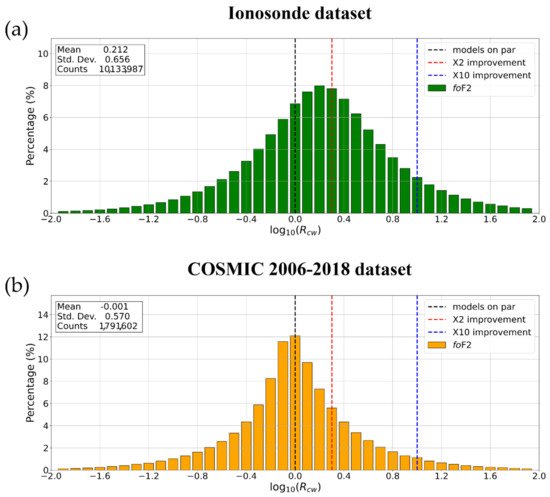
Figure 1. Probability distributions of the residuals’ deviation ratio in a logarithmic scale, log10(Rcw), between IRI and IRTAM models calculated on the (a) entire ionosonde and (b) COSMIC foF2 datasets. The mean, standard deviation, and counts values are reported in the upper left corner of each plot. The dashed vertical lines indicate, respectively, when the models are on par (in black), IRTAM improves IRI by a factor of 2 (in red), and IRTAM improves IRI by a factor of 10 (in blue).
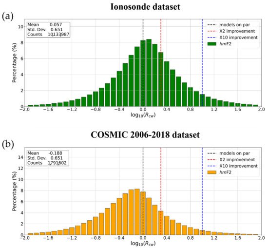
Figure 2. Same as Figure 1 but for hmF2.
The log10(Rcw) distribution shown in Figure 1a is clearly “shifted” towards the positive values. Specifically, the mean value of the distribution equal to +0.212 highlights that overall IRTAM performs better than IRI by a factor of about 1.6 when considering the foF2 ionosonde dataset. Instead, the log10(Rcw) distribution shown in Figure 1b is quite symmetric with respect to the zero value. This fact is strongly supported by the mean value of the distribution, which is equal to −0.001. Therefore, the IRI and IRTAM performances can be considered equivalent when considering the COSMIC foF2 dataset.
The log10(Rcw) distribution shown in Figure 2a is quite symmetric around the zero. Specifically, the mean value of the distribution equal to +0.057 (which corresponds to an improvement factor of about 1.14) highlights that IRTAM and IRI provide quite comparable outputs when considering the hmF2 ionosonde dataset. The log10(Rcw) distribution shown in Figure 46b is clearly “shifted” towards the negative values. Specifically, the mean value of the distribution equal to −0.188 points out that IRI performs better than IRTAM when considering the hmF2 COSMIC dataset by a factor of about 1.5.
The same analysis based on log10(Rcw) distribution was applied by Galkin et al. [18] on a dataset of foF2 values recorded by 59 ionosondes during May–June 2019. They found results very similar to the ones shown in Figure 1a, with IRTAM improving IRI by a factor of about two (about 0.3 in the logarithmic scale of Figure 1). The slight differences are due on the one hand to the fact that to test IRTAM Galkin et al. [18] used only data from assimilated stations, while in this study we used also non-assimilated stations, and on the other hand to the larger extension of our dataset covering different seasons and solar activity levels. Results similar to those of Galkin et al. [18] were obtained also by Vesnin [29] by considering a larger dataset covering one solar cycle, but again using only data from assimilated stations to test the model. Vesnin [29] investigated the IRTAM performance also for hmF2 and found that IRTAM improved IRI by a factor of about 1.8. However, in that analysis the oldest Bilitza et al. [30] hmF2 IRI option was used as comparison. When using the newest Shubin et al. [31] default IRI hmF2 option, we find much lower differences between IRTAM and IRI, thus confirming the very important step forward made by IRI about the hmF2 modeling, as on the other hand recently outlined by different authors [32][33][34].
Figure 1 and Figure 2 confirm the general picture outlined by the analyses described in Section 5, Section 6, Section 7 and Section 8, i.e., the comparison with ionosonde data highlights how IRTAM significantly improves the foF2 prediction made by IRI, while for hmF2 the performances are quite similar between the two models. Since IRTAM assimilates both foF2 and hmF2 from the GIRO network, we would have expected a similar improvement also in the hmF2 prediction. Besides the obvious differences due to the application of the newest Shubin et al. [31] IRI hmF2 default option, two important points need to be highlighted. First, the IRTAM hmF2 description is based on the mapping procedure introduced by Brunini et al. [35], which introduces residuals in the range from −10 to 10 km when compared to the original hmF2 values obtained from the Bilitza et al. [30] formulation. The second point is inherent to the hmF2 derivation from ionograms. In fact, while foF2 is a parameter that is directly obtained from ionograms as the maximum ordinary frequency reflected by the ionosphere, hmF2 has to be derived trough a mathematical inversion procedure that, starting from critical frequencies measured at different virtual heights, allows obtaining the electron density values at real heights [36]. This inversion procedure is sensitive to different possible error sources due to the E-valley presence, the interpretation of the F2-layer cusp made by ARTIST, and in general the quality of the ionogram echo traces. All of these matters may represent possible sources of error, that are estimated in the order of 10 km [37]. From the above considerations, it clearly emerges that to obtain reliable hmF2 values is more difficult than to get foF2 ones, even with data assimilation. This is a point that requires further improvements and refining of both the data assimilation procedure and the measurement technique itself.
The comparison with the F2-layer peak characteristics derived from COSMIC RO showed a general worsening of the IRTAM performances in comparison with the IRI ones. Specifically, the comparison with the COSMIC dataset (Figure 20 and Figure 41) highlighted that IRTAM improves the IRI foF2 and hmF2 predictions mainly in regions characterized by a dense ionosonde network. This suggests the extent to which IRTAM is tied to data assimilated by ionosondes and to the corresponding spatial distribution. Since assimilated data are used by IRTAM to update the coefficients of the spherical harmonic analysis underlying the IRI description, we would have expected that the improvements were not restricted to the ionosondes’ locations but would embrace at least the whole latitudinal sector where assimilated ionosondes are located. Moreover, the IRTAM description should fade towards that of the IRI in regions where the effect of the assimilated data can be considered negligible. These two points are very important, impacting on IRTAM global performances, and need to be deeply investigated for future versions of IRTAM. Currently, IRTAM assimilates data from about 60 GIRO Digisondes. With the ever-increasing number of available Digisondes, able to provide real-time data, and as a consequence of their more homogeneous spatial distribution, a continuous improvement of the IRTAM performance is expected. However, even if in the future the availability of ionosonde data should increase for both the time resolution and the spatial coverage, the fact that IRTAM is so tied to the underlying IRI model (i.e., to the URSI formalism) represents a limit for the improvement and development of IRTAM itself. In fact, IRTAM through NECTAR, to minimize at assimilation sites the mismatch between measured and IRI modeled values, calculates the corrections to be added to the URSI coefficients, but the order of the diurnal and spatial harmonics is left unchanged. This means that steep spatial gradients and fast time variations that are below the limits that can be resolved with the current spatial and temporal resolution of the URSI formalism would not be represented by IRTAM, even with an increased availability of assimilated data. Since steep spatial gradients and fast time variations are customary under specific Space Weather conditions, and the aim of data-assimilation methods is the reliable representation of such conditions, this poses serious limitations for the IRTAM model that its developers should bear in mind in the future.

3. Conclusions

In the present paper, we compared the IRI and IRTAM models; the latter, being a real-time version of IRI, is based on the assimilation of ionosonde measurements. In order to assess the performance of the two models, two different datasets have been considered: (1) foF2 and hmF2 from ground-based ionosonde observations; (2) foF2 and hmF2 from space-based COSMIC RO observations. Through different analyses and comparison methodologies, we highlighted the main performances exhibited by both IRI and IRTAM for different locations and under different diurnal, seasonal, solar and magnetic activity conditions.
The main results of the study are:
  • When ionosonde observations are considered for validation, IRTAM improves significantly the IRI foF2 modeling while it slightly improves the IRI hmF2 modeling.
  • When COSMIC observations are considered for validation, IRTAM improves neither the IRI foF2 modeling nor the IRI hmF2 modeling.
These results highlight that IRTAM, in contrast to most of assimilation models, has ample room for improvement. The points that in our opinion deserve specific attention are: the bad performance of IRTAM when modeling foF2 at low latitudes; the global hmF2 modeling made by IRTAM which is often unreliable, especially in areas far away from the assimilating sites, where the representation made by IRTAM is at times really different from that of the IRI background; the fact that IRTAM performances are too dependent on the assimilated ionosondes location.
The improvement in the near real-time specification of the ionospheric F2-layer peak characteristics is becoming more and more important nowadays for telecommunication purposes and for Space Weather applications in general. For example, Hartman et al. [38] have recently applied IRTAM as the Floating Potential Measurement Unit (FPMU) back-up system that will be used to support the International Space Station (ISS) program. IRTAM foF2 maps were used by Froń et al. [39] to provide global maps of the ionospheric equivalent slab thickness (τ) parameter that are delivered through the GAMBIT Explorer software (http://giro.uml.edu/GAMBIT, accessed on 3 August 2021). An improved real-time specification of τ on a global basis is very important because this parameter describes the shape of the ionospheric electron density profile; thus, an improved specification of τ can help empirical models such as IRI in the description of the profile shape, especially the topside part [40][41][42][43].
Since in the incoming years the applications based on a near real-time specification of the ionospheric conditions will increase in number, an ever more reliable and robust representation of the ionosphere will become of outstanding importance. This is why near real-time data-assimilation models such as IRTAM need continuous improvement and refining, on the one hand to improve the climatological description of the ionosphere made by IRI, and on the other hand to pave the way for a reliable ionospheric weather description.

References

  1. Moldwin, M. An Introduction To Space Weather; Cambridge University Press: Cambridge, MA, USA, 2008.
  2. Cander, L.R. Ionospheric Space Weather; Springer Nature: Cham, Switzerland, 2019.
  3. Schunk, R.W.; Scherliess, L.; Sojka, J.J.; Thompson, D.C.; Anderson, D.N.; Codrescu, M.; Minter, C.; Fuller-Rowell, T.J.; Heelis, R.A.; Hairston, M.; et al. Global assimilation of ionospheric measurements (GAIM). Radio Sci. 2004, 39.
  4. Angling, M.J.; Khattatov, B. Comparative study of two assimilative models of the ionosphere. Radio Sci. 2006, 41.
  5. Decker, D.T.; McNamara, L.F. Validation of ionospheric weather predicted by global assimilation of ionospheric measurements (GAIM) models. Radio Sci. 2007, 42, RS4017.
  6. McNamara, L.F.; Decker, D.T.; Welsh, J.A.; Cole, D.G. Validation of the Utah State University global assimilation of ionospheric measurements (GAIM) model predictions of the maximum usable frequency for a 3000 km circuit. Radio Sci. 2007, 42, RS3015.
  7. McNamara, L.F.; Bishop, G.J.; Welsh, J.A. Assimilation of ionosonde profiles into a global ionospheric model. Radio Sci. 2011, 46, RS2006.
  8. Buresova, D.; Nava, B.; Galkin, I.; Angling, M.; Stankov, S.M.; Coisson, P. Data ingestion and assimilation in ionospheric models. Ann. Geophys. 2009, 52, 235–253.
  9. Nava, B.; Coisson, P.; Radicella, S.M. A new version of the NeQuick ionosphere electron density model. J. Atmos. Sol. Terr. Phys. 2008, 70, 1856–1862.
  10. Nava, B.; Radicella, S.M.; Azpilicueta, F. Data ingestion into NeQuick 2. Radio Sci. 2011, 46.
  11. Pezzopane, M.; Pietrella, M.; Pignatelli, A.; Zolesi, B.; Cander, L.R. Assimilation of autoscaled data and regional and local ionospheric models as input sources for real-time 3-D international reference ionosphere modeling. Radio Sci. 2011, 46, 5009.
  12. Pezzopane, M.; Pietrella, M.; Pignatelli, A.; Zolesi, B.; Cander, L.R. Testing the three-dimensional IRI-SIRMUP-P mapping of the ionosphere for disturbed periods. Adv. Space Res. 2013, 52, 1726–1736.
  13. Shim, J.S.; Kuznetsova, M.; Rastatter, L.; Hesse, M.; Bilitza, D.; Butala, M.; Codrescu, M.; Emery, B.; Foster, B.; Fuller-Rowell, T.; et al. CEDAR electrodynamics thermosphere ionosphere (ETI) challenge for systematic assessment of ionosphere/thermosphere models: NmF2, hmF2, and vertical drift using ground-based observations. Space Weather 2011, 9, S12003.
  14. Pignalberi, A.; Pezzopane, M.; Rizzi, R.; Galkin, I. Effective solar indices for ionospheric modeling: A review and a proposal for a real-time regional IRI. Surv. Geophys. 2018, 39, 125–167.
  15. Pietrella, M.; Pignalberi, A.; Pezzopane, M.; Pignatelli, A.; Azzarone, A.; Rizzi, R. A comparative study of ionospheric IRIEup and ISP assimilative models during some intense and severe geomagnetic storms. Adv. Space Res. 2018, 61, 2569–2584.
  16. Pietrella, M.; Pezzopane, M.; Zolesi, B.; Cander, L.R.; Pignalberi, A. The simplified ionospheric regional model (SIRM) for HF prediction: Basic theory, its evolution and applications. Surv. Geophys. 2020, 41, 1143–1178.
  17. Galkin, I.A.; Reinisch, B.W.; Huang, X.; Bilitza, D. Assimilation of GIRO data into a real-time IRI. Radio Sci. 2012, 47.
  18. Galkin, I.A.; Reinisch, B.W.; Vesnin, A.M.; Bilitza, D.; Fridman, S.; Habarulema, J.B.; Veliz, O. Assimilation of sparse continuous near-Earth weather measurements by NECTAR model morphing. Space Weather 2020, 18, e2020SW002463.
  19. Bilitza, D.; Altadill, D.; Truhlik, V.; Shubin, V.; Galkin, I.; Reinisch, B.; Huang, X. International reference ionosphere 2016: From ionospheric climate to real-time weather predictions. Space Weather 2017, 15, 418–429.
  20. Bilitza, D. IRI the international standard for the ionosphere. Adv. Radio Sci. 2018, 16, 1–11.
  21. Lei, J.; Syndergaard, S.; Burns, A.G.; Solomon, S.C.; Wang, W.; Zeng, Z.; Roble, R.G.; Wu, Q.; Kuo, Y.-H.; Holt, J.M.; et al. Comparison of COSMIC ionospheric measurements with ground-based observations and model predictions: Preliminary results. J. Geophys. Res. 2007, 112, A07308.
  22. Damboldt, T.; Suessmann, P. Information document on the analysis and validity of present ITU foF2 and M (3000) f2 maps. Int. Telecommun. Union 2011. question ITU-R 212-1/3. Available online: http://www.itu.int/md/R07-WP3L-C-0086/en (accessed on 3 August 2021).
  23. Shim, J.S.; Tsagouri, I.; Goncharenko, L.; Rastaetter, L.; Kuznetsova, M.; Bilitza, D.; Codrescu, M.; Coster, A.J.; Solomon, S.C.; Fedrizzi, M.; et al. Validation of ionospheric specifications during geomagnetic storms: TEC and foF2 during the 2013 March storm event. Space Weather 2018, 16, 1686–1701.
  24. Shim, J.S.; Kuznetsova, M.; Rastätter, L.; Hesse, M.; Bilitza, D.; Butala, M.; Codrescu, M.; Emery, B.; Foster, B.; Fuller-Rowell, T.; et al. CEDAR electrodynamics thermosphere ionosphere (ETI) challenge for systematic assessment of ionosphere/thermosphere models: Electron density, neutral density, NmF2, and hmF2 using space based observations. Space Weather 2012, 10, S10004.
  25. Pedatella, N.M.; Yue, X.; Schreiner, W.S. Comparison between GPS radio occultation electron densities and in situ satellite observations. Radio Sci. 2015, 50, 518–525.
  26. Pignalberi, A.; Pezzopane, M.; Tozzi, R.; De Michelis, P.; Coco, I. Comparison between IRI and preliminary Swarm Langmuir probe measurements during the St. Patrick storm period. Earth Planets Space 2016, 68.
  27. Tsagouri, I.; Goncharenko, L.; Shim, J.S.; Belehaki, A.; Buresova, D.; Kuznetsova, M.M. Assessment of current capabilities in modeling the ionospheric climatology for space weather applications: foF2 and hmF2. Space Weather 2018, 16, 1930–1945.
  28. Cai, X.; Burns, A.G.; Wang, W.; Coster, A.; Qian, L.; Liu, J.; Solomon, S.C.; Eastes, R.W.; Daniell, R.E.; McClintock, W.E.; et al. Comparison of GOLD nighttime measurements with total electron content: Preliminary results. J. Geophys. Res. Space Phys. 2020, 125, e2019JA027767.
  29. Vesnin, A.M. Validation of F2 Layer Peak Height and Density of Real-Time International Reference Ionosphere. Master’s Thesis, University of Massachusetts Lowell, Lowell, MA, USA, 2014. Available online: https://ulcar.uml.edu/GAMBIT/Vesnin-Master-thesis-2014.pdf (accessed on 3 August 2021).
  30. Bilitza, D.; Sheik, N.; Eyfrig, R. A global model for the height of the F2-peak using M3000 values from the CCIR numerical map. Telecommun. J. 1979, 46, 549–553.
  31. Shubin, V.N. Global median model of the F2-layer peak height based on ionospheric radio-occultation and ground based digisonde observations. Adv. Space Res. 2015, 56, 916–928.
  32. Arıkan, F.; Sezen, U.; Gulyaeva, T.L. Comparison of IRI-2016 F2 layer model parameters with ionosonde measurements. J. Geophys. Res. Space Phys. 2019, 124, 8092–8109.
  33. Mengist, C.K.; Yadav, S.; Kotulak, K.; Bahar, A.; Zhang, S.-R.; Seo, K.-H. Validation of International Reference ionosphere model (IRI-2016) for F-region peak electron density height (hmF2): Comparison with Incoherent Scatter Radar (ISR) and ionosonde measurements at Millstone Hill. Adv. Space Res. 2020, 65, 2773–2781.
  34. Huang, H.; Moses, M.; Volk, A.E.; Abu Elezz, O.; Kassamba, A.A.; Bilitza, D. Assessment of IRI-2016 hmF2 model options with digisonde, COSMIC and ISR observations for low and high solar flux conditions. Adv. Space Res. 2021.
  35. Brunini, C.; Conte, J.F.; Azpilicueta, F.; Bilitza, D. A different method to update monthly median hmF2 values. Adv. Space Res. 2013, 51, 2322–2332.
  36. Titheridge, J.E. Ionogram Analysis with the Generalised Program Polan, Rep. UAG-93; World Data Center A for Solar-Terrestrial Physics: Boulder, CO, USA, 1985.
  37. Chen, C.F.; Reinisch, B.W.; Scali, J.L.; Huang, X.; Gamache, R.R.; Buonsanto, M.J.; Ward, B.D. The accuracy of ionogram-derived N(h) profiles. Adv. Space Res. 1994, 14, 43–46.
  38. Hartman, W.A.; Schmidl, W.D.; Mikatarian, R.; Galkin, I. Correlation of IRTAM and FPMU data confirming the application of IRTAM to support ISS Program safety. Adv. Space Res. 2019, 63, 1838–1844.
  39. Froń, A.; Galkin, I.; Krankowski, A.; Bilitza, D.; Hernández-Pajares, M.; Reinisch, B.; Li, Z.; Kotulak, K.; Zakharenkova, I.; Cherniak, I.; et al. Towards cooperative global mapping of the ionosphere: Fusion feasibility for IGS and IRI with global climate VTEC maps. Remote Sens. 2020, 12, 3531.
  40. Themens, D.R.; Jayachandran, P.T.; Bilitza, D.; Erickson, P.J.; Häggström, I.; Lyashenko, M.V.; Reid, B.; Varney, R.H.; Pustovalova, L. Topside electron density representations for middle and high latitudes: A topside parameterization for E-CHAIM based on the NeQuick. J. Geophys. Res. Space Phys. 2018, 123, 1603–1617.
  41. Dos Santos Prol, F.; Themens, D.R.; Hernández-Pajares, M.; de Oliveira Camargo, P.; de Assis Honorato Muella, M.T. Linear vary-chap topside electron density model with topside sounder and radio-occultation data. Surv. Geophys. 2019, 40, 277.
  42. Pezzopane, M.; Pignalberi, A. The ESA swarm mission to help ionospheric modeling: A new NeQuick topside formulation for mid-latitude regions. Sci. Rep. 2019, 9, 12253.
  43. Pignalberi, A.; Pezzopane, M.; Themens, D.R.; Haralambous, H.; Nava, B.; Coïsson, P. On the analytical description of the topside ionosphere by NeQuick: Modeling the scale height through COSMIC/FORMOSAT-3 selected data. IEEE J. Sel. Top. Appl. Earth Obs. Remote. Sens. 2020, 13, 1867–1878.
More
Information
Contributor MDPI registered users' name will be linked to their SciProfiles pages. To register with us, please refer to https://encyclopedia.pub/register :
View Times: 669
Revisions: 2 times (View History)
Update Date: 11 Aug 2021
1000/1000