1000/1000
Hot
Most Recent
 +1 point
Convolutional neural network (CNN)-based deep learning (DL) has a wide variety of applications in the geospatial and remote sensing (RS) sciences, and consequently has been a focus of many recent studies.
This paper is the second and final component in a series in which we explore accuracy assessment methods used in remote sensing (RS) (CNN) classification, focusing on scene classification, object detection, semantic segmentation, and instance segmentation tasks. The studies reviewed rarely reported a complete confusion matrix to describe classification error; and when a confusion matrix was reported, the values for each entry in the table generally did not represent estimation of population properties (i.e., represent a probabilistic sample of the map). Some of these issues are not unique to RS DL studies; similar issues have been noted regarding traditional RS classification accuracy assessment, for example by Foody [1] and Stehman and Foody [2].
Building upon traditional RS accuracy assessment standards and practices, a literature review, and our own experiences, we argue that it is important to revisit accuracy assessment rigor and reporting standards in the context of CNNs. In order to spur the development of community consensus and further discussion, we therefore offer an initial summary of recommendations and best practices for the assessment of DL products to support research, algorithm comparison, and operational mapping. In the Background section, we provide an overview of the types of mapping problems to which CNN-based DL is applicable, review established standards and best practices in remote sensing, and summarize current RS DL accuracy assessment approaches. The Recommendations and Best Practices section outlines accuracy assessment issues related to RS DL classification, focusing on issues related to partitioning the data, assessing generalization, assessment metrics, benchmark datasets, and reporting standards.
The geographic arrangement of the partitioning of the three sets of reference data, used for training, validation, and testing, is important, and should be carried out in a manner that supports the research questions posed [3] and produces unbiased accuracy estimates. (US). Figure 1a illustrates simple random chip partitioning, in which image chips are created for the entire study area extent, shown in gray, and then these image chips are randomly split into the three partitions without any additional geographic stratification. Figure 1b illustrates geographically stratified chip partitioning in which chips are partitioned into geographically separate regions. Figure 1c illustrates tessellation stratified random sampling, in which the study area is first tessellated into rectangular regions or some other unit of consistent area.
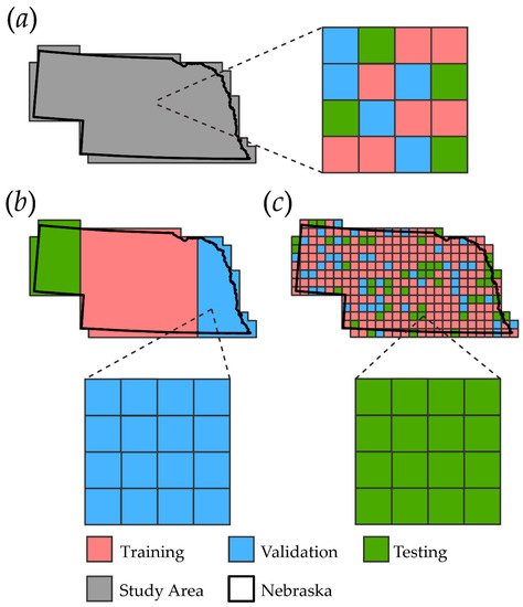
The choice between the three geographic sampling designs described above has potential consequences for accuracy assessment. Both simple random chip partitioning and tessellation stratified random chip partitioning should yield class proportions for each partition similar to those of the entire study area extent. On the other hand, a potential benefit of both the geographically stratified design and the tessellation stratified random sampling design is that the spatial autocorrelation between the partitions is reduced, and thus the accuracy evaluation may be a more robust test of generalization than, for example, simple random chip partitioning. If so, whatever the geographic sampling design, the subsampling within the partitions should be probabilistic so that unbiased population statistics can be estimated.
In developing training, validation, and testing datasets, it is also important to consider the impact of overlapping image chips. Many studies have noted reduced inference performance near the edge of image chips [4][5][6][7]; therefore, to improve the final map accuracy, it is common to generate image chips that overlap along their edges, and to use only the predictions from the center of each chip in the final, merged output. Generally, the final assessment metrics should be generated from the re-assembled map output, and not the individual chips, since using the chips can result in repeat sampling of the same pixels. For the simple random chip sampling described above, this type of separation may not be possible without subsampling, thus making random chip sampling less attractive.
One of the strengths of many RS DL studies is that they explicitly test generalization within their accuracy assessment design, for example by applying the trained model to new data or new geographic regions not previously seen by the model. Conceptually, model generalization assessment is an extension of the geographically stratified chip partitioning method discussed inSection 3.1, except in this case the new data are not necessarily adjacent to or near the training data, and in many cases they involve multiple replications of different datasets. Assessing model generalization is useful both for adding rigor to the accuracy assessment and for providing insight regarding how the model might perform in an operational environment where new training of the model is impractical every time new data are collected. Examples of such generalization tests include Maggiori et al.
In designing an assessment of model generalization, the type of generalization must be defined, and appropriate testing sets must be developed to address the research question. For example, if the aim is to assess how well a model generalizes to new geographic extents when given comparable data, image chips and reference data in new geographic regions will be needed. If the goal is to assess generalization to new input data, then it may be appropriate to select the new data from the same geographic extent that was used to train the original model.
As highlighted in Part 1 of this study [8], there are many inconsistencies in the RS DL literature relating to which assessment metrics are calculated, how they are reported, and even the names and terminology used. DL RS studies have primarily adopted measures common in the DL and computer vision communities and have abandoned traditional RS accuracy assessment metrics and terminology. It is important to report metrics that give end users and other researchers insight into how the model and dataset will perform for the application of interest. Below, we recommend best practices for choosing and reporting accuracy assessment metrics for the four CNN-based problem types with these considerations in mind.
In scene classification, the unit of assessment is a single image or chip. Though the image chips are usually generated from geospatial data, the classified images are not normally mapped or referenced back to a specific spatial location in the assessment. In practice, however, it may be challenging to generate a population matrix for scene classification. Many scene classification benchmark datasets appear to be deliberative samples, and usually by design collect samples that are not in proportion to the likelihood of the class in the population.
An example of a scene classification dataset is DeepSat SAT-6 [9] (available from:https://csc.lsu.edu/~saikat/deepsat/; accessed on 1 July 2021). This dataset differentiates six classes (barren, building, grassland, road, tree, and water) and consists of 28-by-28 pixel image chips derived from National Agriculture Imagery Program (NAIP) orthophotography. A total of 405,000 chips are provided, with 324,000 used for training and 81,000 reserved for testing, as defined by the dataset originators. Figure 2 provides some example image chips included in this dataset.
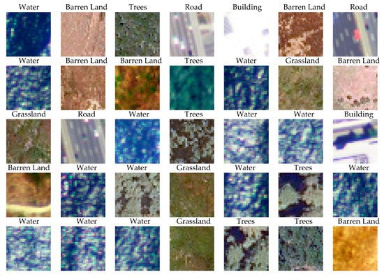
Table 1 summarizes the accuracy of a ResNet-32 CNN-based scene classification in terms of the confusion matrix with values in the table representing the proportions of the classes in the original testing dataset. Thus, the row and column totals represent the prevalence of each class in the classified data and reference data, respectively. Reporting the entire confusion matrix, along with row and column totals, as well as the class accuracy statistics is useful because it allows greater understanding of how the statistics were calculated, as well as the different components of the classification errors. We use DL terms of precision and recall, as well as the traditional RS terms of UA and PA for clarity.
| Reference | Row Total |
Precision (UA) |
F1 | |||||||
|---|---|---|---|---|---|---|---|---|---|---|
| Barren | Building | Grassland | Road | Tree | Water | |||||
| Classification | Barren | 0.2248 | 0.0000 | 0.0006 | 0.0000 | 0.0000 | 0.0000 | 0.2253 | 0.9974 | 0.9943 |
| Building | 0.0000 | 0.0454 | 0.0000 | 0.0000 | 0.0000 | 0.0000 | 0.0455 | 0.9989 | 0.9946 | |
| Grassland | 0.0020 | 0.0000 | 0.1548 | 0.0000 | 0.0002 | 0.0000 | 0.1570 | 0.9861 | 0.9909 | |
| Road | 0.0000 | 0.0004 | 0.0000 | 0.0255 | 0.0000 | 0.0000 | 0.0260 | 0.9819 | 0.9899 | |
| Tree | 0.0000 | 0.0000 | 0.0001 | 0.0000 | 0.1749 | 0.0000 | 0.1750 | 0.9996 | 0.9993 | |
| Water | 0.0000 | 0.0000 | 0.0000 | 0.0000 | 0.0000 | 0.3712 | 0.3712 | 1.0000 | 1.0000 | |
| Column Total | 0.2268 | 0.0459 | 0.1555 | 0.0256 | 0.1751 | 0.3712 | ||||
| Recall (PA) | 0.9912 | 0.9903 | 0.9957 | 0.9981 | 0.9989 | 1.0000 | ||||
Table 2 provides the same data, except this time the columns are normalized to sum to 1.0 (see for example [10]). Because each class has the same column total, this confusion matrix represents a hypothetical case where each class has the same prevalence.
| Reference | Row Total |
Precision (UA) |
F1 | |||||||
|---|---|---|---|---|---|---|---|---|---|---|
| Barren | Building | Grassland | Road | Tree | Water | |||||
| Classification | Barren | 0.0033 | 0.0000 | 0.0010 | 0.0000 | 0.0000 | 0.0000 | 0.0043 | 0.7647 | 0.8633 |
| Building | 0.0000 | 0.0277 | 0.0000 | 0.0000 | 0.0000 | 0.0000 | 0.0277 | 0.9989 | 0.9946 | |
| Grassland | 0.0000 | 0.0000 | 0.2715 | 0.0000 | 0.0007 | 0.0000 | 0.2721 | 0.9975 | 0.9966 | |
| Road | 0.0000 | 0.0003 | 0.0000 | 0.0157 | 0.0000 | 0.0000 | 0.0160 | 0.9803 | 0.9891 | |
| Tree | 0.0000 | 0.0000 | 0.0001 | 0.0000 | 0.6199 | 0.0000 | 0.6200 | 0.9998 | 0.9994 | |
| Water | 0.0000 | 0.0000 | 0.0000 | 0.0000 | 0.0000 | 0.0598 | 0.0598 | 1.0000 | 1.0000 | |
| Column Total | 0.0033 | 0.0280 | 0.2726 | 0.0157 | 0.6206 | 0.0598 | ||||
| Recall (PA) | 0.9912 | 0.9903 | 0.9957 | 0.9981 | 0.9989 | 1.0000 | ||||
Designers of community benchmark datasets, including SAT-6, sometimes do not make it clear whether the proportions of the samples in the various classes represent the prevalence of those classes in the landscape. Thus, it is not clear if Table 1 is truly a population estimate. However, to illustrate how a population estimate can be obtained from these data, we assumed an application in the East Coast of the USA, and obtained a high spatial resolution (1 m2pixels) map of the 262,358 km2Chesapeake Bay region from [11]. In Table 2, the values in the table have been normalized so that the column totals represent the class prevalence values determined from the Chesapeake reference map, and thus, unlike the other two tables, Table 2 provides an estimate of a potential real-world application of the dataset.
This emphasizes that class prevalence affects most summary accuracy metrics, and therefore the prevalence values used are important. Assuming all classes have equal prevalence, as in Table 3, appears to be the standard for RS scene classification. In our survey of 100 papers, five of the 12 studies that dealt with scene classification reported confusion matrices, and all five used this normalization method. However, a hypothetical landscape in which all classes exist in equal proportions is likely to be rare, if it is found at all.
| Reference | Row Total |
Precision (UA) |
F1 | |||||||
|---|---|---|---|---|---|---|---|---|---|---|
| Barren | Building | Grassland | Road | Tree | Water | |||||
| Classification | Barren | 0.9912 | 0.0000 | 0.0037 | 0.0000 | 0.0000 | 0.0000 | 0.9949 | 0.9962 | 0.9937 |
| Building | 0.0000 | 0.9903 | 0.0000 | 0.0019 | 0.0000 | 0.0000 | 0.9922 | 0.9981 | 0.9942 | |
| Grassland | 0.0088 | 0.0000 | 0.9957 | 0.0000 | 0.0011 | 0.0000 | 1.0056 | 0.9902 | 0.9929 | |
| Road | 0.0000 | 0.0097 | 0.0002 | 0.9981 | 0.0000 | 0.0000 | 1.0079 | 0.9902 | 0.9941 | |
| Tree | 0.0000 | 0.0000 | 0.0004 | 0.0000 | 0.9989 | 0.0000 | 0.9993 | 0.9996 | 0.9993 | |
| Water | 0.0000 | 0.0000 | 0.0000 | 0.0000 | 0.0000 | 1.0000 | 1.0000 | 1.0000 | 1.0000 | |
| Column Total | 1.0000 | 1.0000 | 1.0000 | 1.0000 | 1.0000 | 1.0000 | ||||
| Recall (PA) | 0.9912 | 0.9903 | 0.9957 | 0.9981 | 0.9989 | 1.0000 | ||||
As an alternative, some studies only report recall, on the basis that this metric is not affected by prevalence [12][13]. However, Table 2 highlights the potential hazard of such an approach: the classification has values for recall (PA) above 0.99 for all classes, but the barren class has a precision (UA) value of only 0.76. If only recall values are tabulated, the user would be misled as to the reliability of the classification for barren.
The typical output of a DL semantic segmentation is a wall-to-wall, pixel-level, multi-class classification, similar to that of traditional RS classification. For such classified maps, traditional RS accuracy assessment methods, including using a probabilistic sampling scheme to facilitate unbiased estimates of population-based accuracies, and reporting a complete confusion matrix, has direct application. Using traditional terminology, such as UA and PA, would facilitate communication with RS readers, but almost all authors seem to prioritize communication with the DL community and use the computer science or computer vision terms, such as precision and recall. Given that there are so many of these alternative names for the standard RS metrics, perhaps the most important issue is that all metrics should be clearly defined.
Table 4 gives an example confusion matrix for a semantic segmentation, andTable To produce this table, the LandCover.ai multiclass dataset [14] (available fromhttps://landcover.ai/; accessed on 1 July 2021) was classified with an augmented UNet architecture [15], using the training and testing partitions defined by the originators. In Table 4, the values are proportions of the various combinations of reference and classified classes in the landscape, and the column totals represent the class prevalence values. For example, Buildings is a rare class, making up just 0.8% of the reference landscape.
| Reference | Row Total |
Precision (UA) |
F1 Score | |||||
|---|---|---|---|---|---|---|---|---|
| Buildings | Woodlands | Water | Other | |||||
| Classification | Buildings | 0.007 | 0.000 | 0.000 | 0.003 | 0.009 | 0.827 | 0.716 |
| Woodlands | 0.000 | 0.325 | 0.000 | 0.019 | 0.344 | 0.931 | 0.937 | |
| Water | 0.000 | 0.001 | 0.053 | 0.004 | 0.058 | 0.961 | 0.938 | |
| Other | 0.001 | 0.023 | 0.002 | 0.562 | 0.588 | 0.956 | 0.955 | |
| Column Total |
0.008 | 0.349 | 0.056 | 0.588 | ||||
| Recall (PA) | 0.705 | 0.944 | 0.916 | 0.955 | ||||
Table 4 illustrates why the F1 score on its own, without the values of the constituent precision and recall measures, provides only limited information. The F1 scores of Woodlands and Water are almost identical, suggesting the classification performance is basically the same for these two classes. Table 4, however, shows that Water, unlike Woodlands, had a much lower recall than precision.
Surprisingly, although our review of 100 DL papers found the use of many different accuracy metrics, none used some of the more recently developed RS metrics, such as quantity disagreement (QD) and allocation disagreement (AD) suggested by Pontius and Millones [16], which provide useful information regarding the different components of error. For the map summarized in Table 4, the QD was 0.0% and the AD was 5.0%, indicating almost no error is derived from an incorrect estimation of the proportion of the classes; instead, the error derives from the mislabeling of pixels.
Table 5 was derived from [5], which used semantic segmentation to extract the extent of surface mining from historic topographic maps. The accuracy assessment included a geographic generalization component, and was carried out on the mosaicked images, not individual image chips. However, variability in the accuracy of mapping the mining classes and issues of FPs and FNs were captured by precision, recall, and the F1 score. Reporting only the F1 score would obscure the fact that in Geographic Region 4, the much lower accuracy is due to a low recall, whereas the precision is similar to that of the other areas.
| Geographic Region | Precision | Recall | Specificity | NPV | F1 Score | OA |
|---|---|---|---|---|---|---|
| 1 | 0.914 | 0.938 | 0.999 | 0.993 | 0.919 | 0.999 |
| 2 | 0.883 | 0.915 | 0.999 | 0.999 | 0.896 | 0.998 |
| 3 | 0.905 | 0.811 | 0.998 | 0.993 | 0.837 | 0.992 |
| 4 | 0.910 | 0.683 | 0.998 | 9.983 | 0.761 | 0.983 |
CNN-based deep learning can also be used to generate spatial probabilistic models. [17] explored DL for the probabilistic prediction of severe hailstorms, while Thi Ngo et al. If the primary output will be a probabilistic model, probabilistic-based assessment metrics should be reported. Thus, precision (i.e., UA) is not assessed, which can be especially misleading when class proportions are imbalanced.
Object detection and instance segmentation both identify individual objects. Since the number of true negative objects (i.e., objects not part of the category of interest) is generally not defined, reporting a full confusion matrix and the associated OA metric is generally not possible. Nevertheless, reporting the number of TP, TN, FN, and FP, along with the derived accuracy measures typically used—precision, recall, and F1 (e.g., [18])—ensures clarity in the results.
A further complication for object detection is that there is normally a range of confidence levels in the detection of any single object. In the context of object detection, however, the AUC PR is normally referred to as average precision (AP), and/or mean average precision (mAP). The second component of object probability, the delineation of the object, is usually quantified in terms of the IoU of the reference and predicted masks or bounding boxes. However, because the choice of a threshold is usually arbitrary, a range of thresholds may be chosen, for example, from 0.50 to 0.95, with steps of 0.05, which would generate 10 sets of object detections, each with its own P-R curve and AP metric.
Unfortunately, there is considerable confusion regarding the AP/mAP terminology. First, these terms may be confused with the average of the precision values in a multiclass classification (e.g. a semantic segmentation). Second, mAP is generally used to indicate a composite AP, for example, typically averaged over different classes [19][20][21], but also sometimes different IoU values [22]. However, because of inconsistencies in the usage of the terms AP and mAP in the past, some sources (e.g., [23]) no longer recommend differentiating between them, and instead use the terms interchangeably.
Because of the lack of standardization in AP and mAP terminology, it is important for accuracy assessments to clearly report how these accuracy metrics were calculated, for example, specifying the IoU thresholds used. Adding subscripts for IoU thresholds, if thresholds are used, or BB or M to indicate whether the metrics are based on bounding boxes or pixel-level masks, can be an effective way to communicate this information (for example, APBBor IoUM). [24] used both superscripts and subscripts to differentiate six AP metrics derived from bounding box and pixel-level masks, as well as three different sizes of objects (small, medium, and large).
In reporting object-level data, it is important to consider whether a count of features or the area of features is of interest. For example, a model may be used to predict the number of individual trees in an image extent. In such a case, it would be appropriate to use the numbers of individuals as the measurement unit. However, if the aim is to estimate the area covered by tree canopy, then it would be more appropriate to use assessment metrics that incorporate the relative area of the bounding boxes or masks.
A variety of benchmark geospatial datasets are available to test new methods and compare models. [25] provide an extensive comparison of benchmark datasets. Despite the range of publicly available benchmark datasets, there are notable gaps in the available data. and/or data are limited, and there is also generally a lack of non-image benchmark datasets, such as those representing LiDAR point clouds, historic cartographic maps, and digital terrain data, as noted in our prior studies [5][6].
Benchmark datasets and the associated metadata inherently constrain the potential for rigorous accuracy assessment, depending on the nature of the data and, crucially, how they are documented. Benchmark datasets in many cases provide pre-determined protocols for accuracy assessment. Therefore, it is particularly helpful if benchmark datasets support best practices, as described below: If the dataset is meant to support the assessment of model generalization to new data and/or geographic extents, the recommended validation configuration should be documented.
In order to improve consistency between studies, replication capacity, and inference potential, it is important to report, in detail, the research methods and accuracy assessment metrics. Here, we provide a list of reporting standards and considerations that will promote clarity for interpretation and replication of experiments.
First, comparison of new methods and architectures is hindered by the complexity of hyperparameter optimization and architecture design [26][27][28][29]. However, due to lengthy training times, computational demands, and a wide variety of hyperparameters and architecture changes that can be assessed, such systematic experimentation is currently not possible for CNN-based DL [26][27][28][29][30]. When new algorithms or methods are proposed, it is common to use existing machine learning or DL methods as a benchmark for comparison; however, we argue that such comparisons are limited due to an inability to optimize the benchmark model fully [31][32]. [32] suggest that reported improvements when using new algorithms and architectures are often overly optimistic due to inconsistencies in the input data, training process, and experimental designs and because the algorithm to which the comparison is being made was not fully optimized.
This issue is further confounded by the lack of a theoretical understanding of the data abstractions and generalizations modeled by CNNs [33]. For example, textural measures, such as those derived from the gray level co-occurrence matrix (GLCM) after Haralick [34], have shown varying levels of usefulness for different mapping tasks; however, one determinant of the value of these measures is whether or not the classes of interest have unique spatial context or textural characteristics that allow for greater separation [35][36][37][38]. Building on existing literature, a better understanding of how CNNs represent textural and spatial context information at different scales could potentially improve our general understanding of how best to represent and model textural characteristics to enhance a wide range of mapping tasks. Furthermore, improved understanding could guide the development of new DL methods and architectures.
Accuracy estimates are usually empirical estimates of map properties, and as with all statistical estimates, they have uncertainties. , we suggest that confidence intervals be reported where possible. For example, confidence intervals can be estimated for overall accuracy [39] and AUC ROC [40] or multiple model runs can be averaged to assess for variability. Such information can be informative, especially when only small differences in assessment metrics between models are observed.
For example, accuracy assessment methods generally assume that all pixels will map perfectly to the defined classes and that feature boundaries are well-defined. The impact of landscape complexity and heterogeneity should also be considered when designing accuracy assessment protocols and interpreting results. For example, heterogenous landscapes may prove more difficult to map in comparison to more homogeneous landscapes, resulting from more boundaries, edges, class transitions, and, potentially, mixed pixels or gradational boundaries [41][42]. Accounting for mixed pixels, gradational boundaries, difficult to define thematic classes, and the defined minimal mapping unit (MMU) are complexities that exist for all thematic mapping tasks, including those relying on DL, which highlight the need for detailed reporting of sample collection and accuracy assessment methods [8][1][2][43][41][44][45][46][47][48].
Such findings can inform DL researchers as to existing mapping difficulties and research needs, which classes are most difficult to differentiate, and which classes are most important to map for different use cases. We argue that considering the existing literature, methods, and complexities relating to specific mapping tasks or landscape types can offer guidance for knowledge gaps and research needs to which DL may be applicable. Similarly, the current body of knowledge offers insights for extracting information from specific data types. For example, extracting information from true color or color infrared aerial imagery with high spatial resolution, limited spectral resolution, and variability in illuminating conditions between images is an active area of research in the field [14][49][50][51][52][53].