A Multi-Level Optimization Approach

Version	Summary	Created by	Modification	Content Size	Created at	Operation
1		Joseph Daniel Pineda-Sandoval	+ 3020 word(s)	3020	2021-09-29 05:56:47	\|
2	Done	Jason Zhu	Meta information modification	3020	2021-10-07 06:03:27	\| \|
3	Done	Jason Zhu	Meta information modification	3020	2021-10-28 11:34:49	\|

This entry is adapted from the peer-reviewed paper 10.3390/en14185806

Researchers optimizes Chlorine Booster Stations (CBS) location on a network with two main objectives; (1) to deliver minimal Free Residual Chlorine (FRC) throughout all demand nodes according to country regulations, and (2) to reduce day chlorine mass concentration supplied in the system by applying an hour time pattern in CBS, consequently associated economic, energy and environmental impacts complying with regulatory standards

water distribution systems EPANET water quality Chlorine booster Chlorine distribution social and environmental impacts genetic algorithms particle swarm optimization

1. Introduction

Water utilities properly treat water for common usage and in some cases for drinking. The practices of most water utilities in developing countries are to disinfect water with chlorine, due to the low cost and easy production ^[1]^[2]^[3]^[4]^[5]. Chlorination is the method at which water is disinfected from viruses and bacteria. This process occurs in the Drinking Water Treatment Plant (DWTP) and guarantees safe water until the last consumer node. The problem derived from chlorine decay over time due to WDN conditions which many of them does not count with Chlorine Booster Stations (CBS) a way of redistributing doses of disinfectant. Water utilities to supply the minimum Free Residual Chlorine (FRC) at the end of the WDN, add elevated doses of disinfectant at the exit of the DWTP ^[6]. Reducing chlorine demand from water utilities derives less chlorine manufacture and energy consumption, and a better perception from consumers in tap water safety improves the quotes collection for water utilities; furthermore, there will be a reduction in bottled water and thus a lower environmental impact ^[7]. This is important because chlorine gas is commonly manufactured by electrolysis which in some of its variances uses at least 3560 kWh/Ton Cl₂ ^[8]. Regulations in the United States of America (USA) established the maximum residual disinfectant level as 4.0 mg/L, above this level exist the potential risk of eyes/nose irritation and possible stomach discomfort, also a minimum of 0.2 mg/L which guarantee disinfection of pathogenic bacteria ^[9]; while there exists different regulations for each country, the World Health Organization (WHO) recommends a maximum FRC concentration of 0.5 mg/L and minimum of 0.2 mg/L in the WDN to guarantee the disinfection of water on consumer nodes.

Low disinfectant concentration at DWTP can result in a poor distribution of chlorine and/or fast chlorine decay ^[10]. This concentration scenario has been responsible for a significant number of waterborne disease outbreaks, associated with microorganisms such as E. coli, norovirus, giardia, cryptosporidium amongst others ^[11]^[12]. Chlorine decay can occur due to the loss of physical integrity caused by diverse factors, such as (a) water main breaks/repair sites, (b) uncovered reservoirs or covered storage tanks with structural deficiencies, (c) cross connections when inappropriately installed, (d) inadequately maintained backflow prevention devices and the loss of hydraulic integrity as incapability to maintain desirable water flow, water pressure, and high residence of water in pipes (i.e., water age) ^[13]^[14].

The loss of physical integrity in pipelines allows the entrance of microorganisms and other elements that increase chlorine decay ^[13]. As a result, layers of microorganisms attached to the pipeline walls acting as microbial pathogens reservoirs known as biofilms, representing a health risk ^[15]. Even after treatment, the disinfectant in water can interact within algal organic matter in reservoirs and produce by-products ^[16]. Organic matter from biofilms interact with disinfectant and produce carcinogenic by-products, a chemical group known as Trihalomethanes (TTHM’s) ^[17]. The identification of these by-products was studied 30 years ago as potentially harmful chlorinated organic material, the most common by-products being chloroform and haloforms. However, the risk of drinking these unintentional by-products is hard to compare against non-disinfected water ^[18]^[19], as in recent years the studies on disinfectant by-products have focused on the most toxic. After the large amount of disinfection by-products discovered, it is necessary to prioritize a new common data format and data to archive, extract and classify known by-products from those that have not been studied ^[20]^[21]^[22]^[23]. The consumption of drinking water with high concentrations of TTHM’s is associated with bladder cancer, of which at least 47% predominate in those who drank tap water with doses higher than 50 µg/L of TTHM’s, compared with those with 5 µg/L or less ^[24].

2. Current Studies

The evaluations for robustness validation in Case Study 1 were made using PSO and GA with the number of CBS that water utilities can build, considered to be two. Evaluation performances are shown in statistical analysis within 100 simulations. CBS represents the number of boosters stations proposed by the algorithm. CBS simulation reached represents the number of times which that number of CBS was proposed during the 100 simulations. Finally, CBS ID represents the name associated with the node where CBS is proposed.

2.1. Statistical Results from GA Location for Case Study 1

For robustness validation of the optimization process, 100 GA simulations were performed. The results showed that 49% of 100 simulations made by GA guaranteed the minimal FRC in all nodes. The best locations for CBS are presented in Table 1. It is considered that the most important CBS is located at node 1 with 100% of the simulations proposing a CBS in that node. The second node, proposed by GA to establish a CBS, was the water supply tank in node 26, with 72% of frequency. Other nodes appeared and a result from the usage of 3 or more CBS associated with nodes 14 and 29 and the remaining nodes were dismissed because of their low frequency.

Table 1. Number of CBS distribution and frequency proposed by GA technique, (Statistical GA Location at Case 1).

CBS	CBS Simulation Reached	CBS ID
2	56	Node 1, Tank
3	30	Node 1, Node 14, Tank
4	13	Node 1, Node 14, Node 29, Tank
5	1	Node 1, Node 29, Node E, Node 32
Total	100 ¹

2.2. Statistical Results from PSO location for the Case Study 1

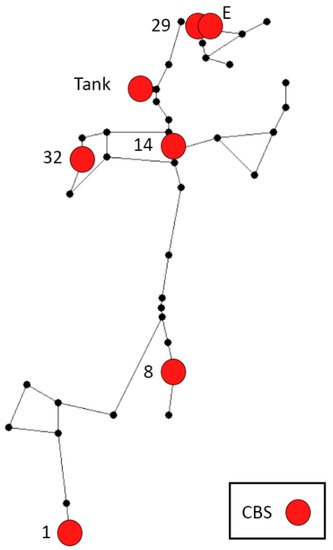
From PSO simulation was obtained 100 simulations to obtain the best locations for CBS (Table 2). Results have shown higher frequency at the pump station, corresponding to node 1 and the tank, and the others were dismissed due to their low frequency (Figure 1).

Figure 1. CBS location mostly proposed in Case Study 1.

Table 2. Number of CBS distribution and frequency proposed by PSO, (statistical PSO location at Case 1).

CBS	CBS Reached	CBS ID
2	71	Node 1, Tank
3	19	Node 1, Node 14, Tank
4	8	Node 1, Node 14, Node 29, Tank
5	2	Node 1, Node 14, Node 29, (Node E or Node 8)
Total	100 ¹

Then, the best and worst individuals are reported by the frequency of CBS ID. It is considered the best individual from the 100 simulations with no penalty in the FF and FRC higher than 0.2 mg/L for all consumer nodes. Thus, the best individual has the FF nearer to the value of one. The individuals with the lower penalty reported CBS location in node 1 (proposed by 100% of simulations) and Water Distribution Tank (proposed by 67% of the simulations). As the main objective was to find the best location for guaranteeing the minimal FRC above all the consumer nodes concentrations, zero or one were selected for representing whether there is chlorine injection in the node or not during the string coding in GA. The optimization algorithm in default settings that worked better on these 100 simulations was PSO.

2.3. Scheduling in CBS Results from GA and PSO

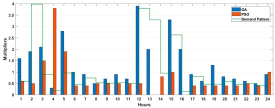
The best location was obtained previously for CBS in Net Example 2. This step aims to determine the schedule pattern dosing to reduce the amount of chlorine per day, thus reducing the economic and environmental impact from water utilities applying the FF2. The optimization consisted in adding hourly multipliers in patterns assigned to the CBS previously selected or presented in the WDN. The patterns are considered by 24 h and if the simulation is larger, then the cycle is repeated. The initial concentration of CBS is considered to be 1 mg/L, so the multiplier would range between regulation values until maintaining the FRC in all consumer nodes and reducing the total dosage of chlorine per day. Thus, those patterns with the lowest dosage per day and the minimal penalty for the tank in Figure 2. The upper boundary is considered as the maximum chlorine allowed of 4 mg/L and a minimal of 0.2 mg/L, inducing multipliers between those values.

Figure 2. Tank CBS pattern chlorine injection for GA vs. PSO.

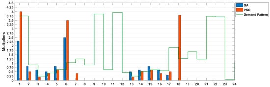
The statistical analysis of scheduling the concentrations in the CBS from the GA shows an average DEL of 0.42 mg/L for 100 simulations and 73% of the simulations reduced the penalty to zero, and only 14% were greater than the average value of the penalty. The best values are obtained in simulation 32 with a zero-penalty value and the lower dosage per day of 1762.75 mg/L. As node 1 works as a pump station, a pattern is assigned (Figure 3), and the injection in WDN from 6 to 12 h and from 17 to 24 h are dismissed because the pump does not supply water in these hours thus chemical neither. The consideration is that at those hours water is distributed from the tank and not from the pump.

Figure 3. Node 1 CBS pattern chlorine injection from GA vs. PSO.

Considering the same procedure, the scheduling in CBS results from PSO shows in the statistical analysis of 100 simulations for PSO that 100% of the simulations reduced the penalty to zero. Therefore, the best value focuses on such individuals that dose the minimal mass of chlorine per day, or with zero-penalty value, and the lower dosage of 1279 g/day was founded in the simulation number 27. As the node 1 works as a pump station, an hourly pattern was assigned and there is no chlorine injection to the WDN from 6 to 12 and from 18 to 24 h.

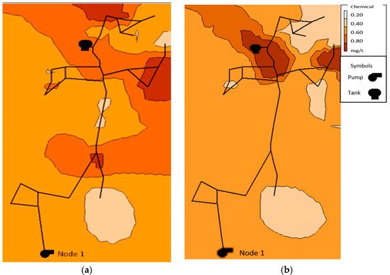
Both cases use two CBS obtained by solutions from GA and PSO, respectively. This condition guaranteed the minimal concentration of FRC in the scenario of the last 24 h. Figure 4 shows chlorine distribution at hour 72 of simulation, which is considered for dismissing initial water quality conditions and mixing tank effects ^[25].

Figure 4. FRC distribution at hour 72. (a) Generated by the GA solution. (b) Generated by the PSO solution.

Both results obtained a full coverage with at least 0.2 mg/L. It was observed that PSO proposes lower concentrations of chlorine (total injected chlorine at 1279.00 g/day while GA maintains higher concentrations (total injected chlorine at 1762.75 g/day. Additionally, while GA have the higher concentration of chlorine injection, this has the lower standard deviation of FRC among the network nodes (Table 3).

Table 3. Statistical values of FRC (mg/L) from the last 24 h of simulation in all nodes.

Metaheuristic Technique	Mean	Standard Deviation Mean	Min	Max
GA	0.64	0.25	0.20	2.24
PSO	0.53	0.43	0.20	3.87

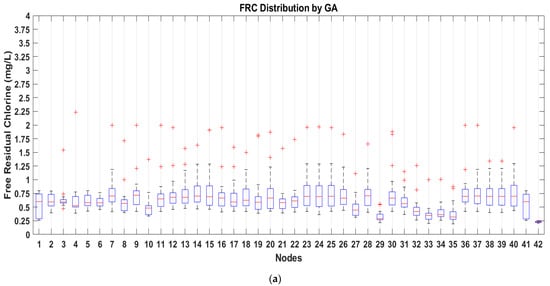
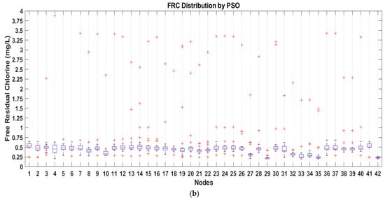
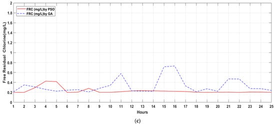
The results of FRC for the last 24 h of simulation for each optimization program showed that GA for most parts of the day remained between the values of 0.25 and 0.8 mg/L (Figure 5a), while PSO obtained 75% of values equal or lower of 0.6 mg/L (Figure 5b), plot interpretation can be made with Figure 6. Therefore, PSO represents a minor concentration of FRC but still guarantees regulated values, which would help reduce corrosion in pipelines and reduce the TTHM’s formations. Both algorithms can solve the problem through trial and error, however the current methodology does not allow parallel processing and as consequence needs more time and computational resources for getting the final solution.

Figure 5. (a) FRC Distribution concentrations on the nodes of the WDN for the solution by GA. (b) FRC Distribution concentrations on the nodes of the WDN for the solution by PSO.

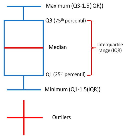
Figure 6. Box and whisker symbology.

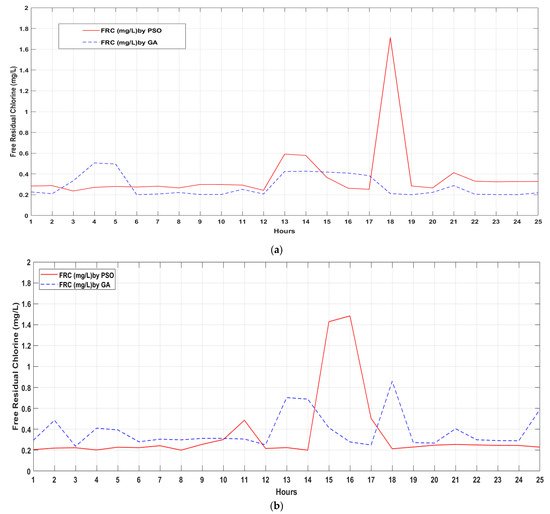
GA results show that even if the concentration injected per day is minimized, nodes; 30, 34 and 36 (Figure 1 and Figure 5a), which are farther from the initial distribution point, reach the minimal FRC. In the same way, the FRC concentration in those nodes guarantees the minimal concentration obtained by the method PSO in the last 24 h of simulation (Figure 5b). FRC analysis from nodes 30, 34 and 36 is presented in Figure 6a–c, respectively.

Figure 6. (a) FRC concentrations on the farthest modes from the initial distribution (node 30). Last day of simulation obtained for GA and PSO. (b) FRC concentrations on the farthest modes from the initial distribution (N = node 34). Last day of simulation obtained for GA and PSO. (c) FRC concentrations on the farthest modes from the initial distribution (node 36). Last day of simulation obtained for GA and PSO.

2.4. CBS Location and Dosage Results for the Case 1

Multiple analyses were simulated through two different optimization models (GA, PSO). Solutions showed by the optimization models selected the best location for two CBS is near the principal water sources as the pump station in node 1 and node 26 (Water Supply Tank).

Finally, the total mass injected by the CBS obtained with GA and PSO is calculated and compared with those described in the literature review (Table 4). It can be observed that the total dosage of chlorine injected per day is 1279 g/day for PSO even if the injection patterns are higher at some hours. Additionally, PSO obtained a value of 66 g/day difference with the minimal dosage obtained from Hybrid optimization with solver Harmony Search. As the results of evaluations show that PSO obtained the significant number of feasible solutions in the optimization model for CBS location and scheduling pattern chlorine injection.

Table 4. Comparison of the total mass injected by the CBS obtained with GA and PSO with those described in the literature review for Case 1.

Author and Year	Optimization Technique	Selected Nodes	Mean Dosage (mg/L)	Total Dosage (g/Day)
This paper	GA (Case study 1)	Node 1 Node 25	0.79 1.29	1762
This paper	PSO (Case study 1)	Node 1 Tank	1.13 0.76	1279
Boccelli et al., 1998 ^[26]	¹ Linear Programming. Case IV	Link 1 (A) Link 8 (B) Link 9 (C) Link 38 (D) Link 34 (E) Link 29 (F)	318.8 ¹ 4.65 ¹ 2089.6 ¹ 0.01 ¹ 0.6 ¹ -	3475
Propato and Uber, 2004 ^[25]	Linear Least Squares	Link 1 (A) Link 29 (F)	0.26 0.22	1321
Ayvaz et al., 2018 ^[27]	Hybrid optimization with solver Harmony Search	Node 2 Node 25	0.517 0.349	1213

2.5. CBS Location Results for the WDN “SF812” in Case Study 2

The WDN “SF812” was evaluated with PSO since previous analysis showed it is more efficient with default settings in the Optimization Matlab Toolkit. It achieved 100% minimal FRC coverage and 71% achieved the goal of established a CBS number decision, which guarantee a reliable solution.

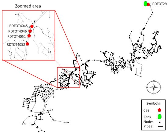
The optimization of chlorine concentration was made considering the CBS location after a time simulation of 232 h. Results proposed 4 CBS in the WDN: RDTOT4045, RDTOT4046, RDTOT4051, RDTOT4052 and a CBS located after the DWTP, in node RDTOT29 (Figure 7). The minimal distance between the nearer CBS is 9.45 m, meaning the more distant is 64.77 m from each other in this group of CBS. The concentration supplied by each node is the maximum allowed of 4 mg/L in each CBS, which could be due to the severe conditions of chlorine decay in the WDN. The CBS locations are in the southwest of the WDN, which represents more than half of the way until the last node supplied by the tank since the sector after this area has the higher quality problems in the WDN.

Figure 7. CBS location proposed by the PSO simulation in Case 2.

Figure 8 shows the chlorine distribution at hour 288 of simulation, with non-scheduled CBS with 4.0 mg/L at each one, a coverage in all consumer nodes with minimal FRC, except (1) the source, which is before the chlorine station, and (2) node RDTOT51 which closes sector with a valve in that point.

Figure 8. FRC distribution at hour 288 with CBS with fixed pattern dosage of 4 mg/L per hour.

The proposal of scheduling with PSO (Figure 9) received a penalty DEL = 5.33 mg/L and a total chlorine injection in the net of 21,912.82 g/day. This increment in the chlorine injection is because of the increment in the range of chlorine injection, and the objective of covering all consumer nodes with minimal FRC, the mean standard deviation is 0.042 mg/L, in the last 24 h for all nodes, and non-consumer nodes with base demand of zero were dismissed. As shown in Figure 9, node RDTOT29 distributes chlorine 24 h per day while auxiliary CBS focuses on distributing chlorine during the night period. This happens because during the night consumers are sleeping, and the water remains in the pipe system, so the water is mainly taken from the pipelines rather than the tank.

Figure 9. Chlorine injection dosage by pattern hour between the limits of 0.2 and 5 mg/L.

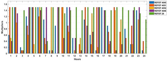
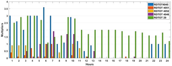
Then, to obey local regulations from Mexico ^[28], chlorine limit ranges are proposed between 0.2 and 1.5 mg/L for scheduling simulations in Figure 10. Thus, multipliers patterns are assigned to hourly distribution to the initial injection of 1 mg/L. Results show a dosage injection of 14.52 kg/day of chlorine mass, and DEL = 57.85 mg/L. In the chlorination pattern, it can be observed that the quantity of chlorine that can be injected most of the time in RDTOT29 was reduced, and auxiliary CBS works at the top amount of chlorine allowed. This is due to severe conditions in the network associated with chlorine decay coefficients.

Figure 10. Pattern time dosage in Case 2 between local regulations.

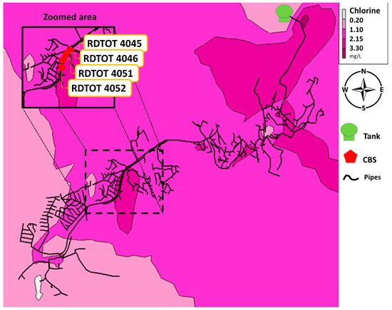
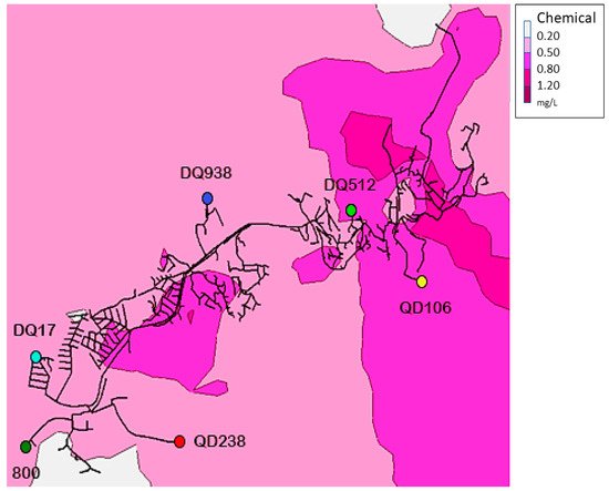
Figure 11 shows the contour plot of time statistical mean FRC applied from the pattern in CBS, as shown in Figure 15. As the network remains between FRC Mexican regulations, some points at the end (south-east) of the network which do not comply with the minimum values. Thus, critical nodes are presented (Table 5) and evaluated. These nodes were selected due to their characteristics as elevation, position, and flow velocity from the nearest link.

Figure 11. FRC distribution in Case 2 by scheduling hourly dosage pattern obtained in Figure 15.

Table 5. Characteristics of critical nodes in Case 2.

Nodes ID	Elevation (m)	Node Demand (L/s)	Pressure (m)
‘DQ512’	2071.38	0.04	31.63
‘QD106’	2021.63	0.02	43.11
‘DQ938’	2059.97	0.06	17.87
‘800’	1998.83	0.06	62.68
‘QD238’	1966.00	0.22	94.84
‘DQ17’	2035.64	0.14	20.86

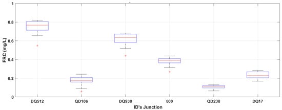
The obtained results from the pattern limit injection between 0.2 and 1.5 did not guarantee the minimum FRC required in the net due to severe conditions of the network as topography and initial water conditions. However, the application represents a significant improvement to the initial conditions of the network, maintaining a mean FRC of 0.71 mg/L, as well from the total simulation time guaranteed the nodes the FRC upper 0.2 mg/L in 95.85%, as we can see in statistical results (Table 6). From nodes DQ238 and QD106 where box and whiskers plot for critical nodes (Figure 17) minimal FRC could not be obtained; most problems are related to uneven surfaces and low demand, which translates into long-time water stagnation in pipes and CBS would not be a feasible solution. Implementation of CBS in the WDN improves the water quality with a better chlorine distribution and, as a collateral effect, diminishes the risk of disinfection by-product formation.

Figure 12. Box and whisker FRC distribution in Case 2 for critical nodes.

Table 6. Statistical values of FRC (mg/L) from the last 24 h of simulation in all nodes.

Metaheuristic Technique	Mean	Std Deviation Mean	Min	Max	Hours Upper 0.2
PSO	0.71	0.25	0	1.5	95.85%

References

Chang, D.; Allen, D.T. Minimizing Chlorine Use: Assessing the Trade-offs Between Cost and Chlorine Reduction in Chemical Manufacturing. J. Ind. Ecol. 1997, 1, 111–134.
Burch, J.; Thomas, K.E. An Overview of Witter Disinfection in Developing Countries and the Potential for Solar Thermal Water Pasteurization; National Renewable Energy Laboratory: Golden, CO, USA, 1998.
Arnold, B.F.; Colford, J.M. Treating Water with Chlorine at Point-of-Use to Improve Water Quality and Reduce Child Diarrhea in Developing Countries: A Systematic Review and Meta-Analysis. Am. J. Trop. Med. Hyg. 2007, 76, 354–364.
Fitzmaurice, A.G.; Mahar, M.; Moriarty, L.F.; Bartee, M.; Hirai, M.; Li, W.; Gerber, A.R.; Tappero, J.W.; Bunnell, R.; GHSA Implementation Group. Contributions of the US Centers for Disease Control and Prevention in Implementing the Global Health Security Agenda in 17 Partner Countries. Emerg. Infect. Dis. 2017, 23, S15–S24.
Reiff, F.M.; Roses, M.; Venczel, L.; Quick, R.; Witt, V.M. Low-Cost Safe Water for the World: A Practical Interim Solution. J. Public Health Policy 1996, 17, 389–408.
Turgeon, S.; Rodriguez, M.J.; Thériault, M.; Levallois, P. Perception of drinking water in the Quebec City region (Canada): The influence of water quality and consumer location in the distribution system. J. Environ. Manag. 2004, 70, 363–373.
Delpla, I.; Legay, C.; Proulx, F.; Rodriguez, M.J. Perception of tap water quality: Assessment of the factors modifying the links between satisfaction and water consumption behavior. Sci. Total Environ. 2020, 722, 137786.
Noval Goméz, L. El Cloro Producción e Industria. Master’s Thesis, Universidad Nacional de Educación a Distancia, Madrid, Spain, 2017.
United States Environmental Protection Agency. National Primary Drinking Water Regulations. Available online: https://www.epa.gov/ground-water-and-drinking-water/national-primary-drinking-water-regulations#Disinfectants (accessed on 9 May 2021).
Bertelli, C.; Courtois, S.; Rosikiewicz, M.; Piriou, P.; Aeby, S.; Robert, S.; Loret, J.-F.; Greub, G. Reduced Chlorine in Drinking Water Distribution Systems Impacts Bacterial Biodiversity in Biofilms. Front. Microbiol. 2018, 9, 2520.
Besner, M.-C.; Prévost, M.; Regli, S. Assessing the public health risk of microbial intrusion events in distribution systems: Conceptual model, available data, and challenges. Water Res. 2010, 45, 961–979.
Craun, G.F. Waterborne Diseases in the US; CRC Press: Boca Raton, FL, USA, 2018; ISBN 1-351-08611-1.
Mora-Rodríguez, J.; López-Jiménez, P.A.; Ramos, H.M. Intrusion and leakage in drinking systems induced by pressure variation. J. Water Supply Res. Technol. 2012, 61, 387–402.
Al-Jasser, A. Chlorine decay in drinking-water transmission and distribution systems: Pipe service age effect. Water Res. 2007, 41, 387–396.
Morvay, A.A.; Decun, M.; Scurtu, M.; Sala, C.; Morar, A.; Sarandan, M. Biofilm formation on materials commonly used in household drinking water systems. Water Supply 2011, 11, 252–257.
Dong, F.; Lin, Q.; Li, C.; He, G.; Deng, Y. Impacts of pre-oxidation on the formation of disinfection byproducts from algal organic matter in subsequent chlor(am)ination: A review. Sci. Total. Environ. 2020, 754, 141955.
Ramos-Martínez, E. Biofilms en los sistemas de distribución de agua potable: Aproximación basada en sistemas multi-agente. In Proceedings of the Formación de Biopelículas y su Impacto en Los Sistemas de Conducción de Agua, Valencia, Spain, 14 September 2018.
Richardson, S.D.; Plewa, M.J. To regulate or not to regulate? What to do with more toxic disinfection by-products? J. Environ. Chem. Eng. 2020, 8, 103939.
Poleneni, S.R. Global disinfection by-products regulatory compliance framework overview, disinfection by-products in drinking water: Detection and treatment. In Disinfection By-Products in Drinking Water; Prasad, M.N.V., Ed.; Butterworth-Heinemann: Oxford, UK, 2020; pp. 393–411. ISBN 978-0-08-102977-0.
Bellar, T.; Lichtenberg, J.; Kroner, R. The Occurrence of Organohalides in Chlorinated Drinking Waters. Am. Water Work. Assoc. 1974, 66, 703–706.
Rook, J.J. Haloforms in Drinking Water. Am. Water Work. Assoc. 1976, 68, 168–172.
Wawryk, N.J.; Craven, C.; Blackstock, L.K.J.; Li, X.-F. New methods for identification of disinfection byproducts of toxicological relevance: Progress and future directions. J. Environ. Sci. 2020, 99, 151–159.
Frimmel, F.H.; Jahnel, J.B. Formation of Haloforms in Drinking Water. In Haloforms and Related Compounds in Drinking Water; Nikolaou, A.D., Ed.; Springer: Berlin/Heidelberg, Germany, 2003; pp. 1–19. ISBN 978-3-540-44997-3.
Li, X.-F.; Mitch, W.A. Drinking Water Disinfection Byproducts (DBPs) and Human Health Effects: Multidisciplinary Challenges and Opportunities. Environ. Sci. Technol. 2018, 52, 1681–1689.
Propato, M.; Uber, J.G. Linear Least-Squares Formulation for Operation of Booster Disinfection Systems. J. Water Resour. Plan. Manag. 2004, 130, 53–62.
Boccelli, D.L.; Tryby, M.E.; Uber, J.G.; Rossman, L.A.; Zierolf, M.L.; Polycarpou, M.M. Optimal Scheduling of Booster Disinfection in Water Distribution Systems. J. Water Resour. Plan. Manag. 1998, 124, 99–111.
Ayvaz, M.T.; Geem, Z.W. Optimum design of the booster chlorination systems by using hybrid HS-Solver optimization technique. Pamukkale Univ. J. Eng. Sci. 2018, 24, 444–452.
S.S.A. Norma Oficial Mexicana NOM-127-SSA1-1994. Salud Ambiental, Agua Para Uso y Consumo Humano-Limites Permisibles de Calidad y Tratamientos a que Debe Someterse el Agua Para su Potabilización; Citing a Federal Regulation in Mexico, 2000.

© Text is available under the terms and conditions of the Creative Commons Attribution (CC BY) license; additional terms may apply. By using this site, you agree to the Terms and Conditions and Privacy Policy.

Upload a video for this entry

Information

Subjects: Engineering, Civil

Contributor MDPI registered users' name will be linked to their SciProfiles pages. To register with us, please refer to https://encyclopedia.pub/register :

Joseph Pineda-Sandoval

View Times: 402

Update Date: 28 Oct 2021

Table of Contents

Video Upload Options

Confirm