1000/1000
Hot
Most Recent
 +1 point
Non-intrusive load monitoring (NILM) is a process of estimating operational states and power consumption of individual appliances, which if implemented in real-time, can provide actionable feedback in terms of energy usage and personalized recommendations to consumers. Intelligent disaggregation algorithms such as deep neural networks can fulfill this objective if they possess high estimation accuracy and lowest generalization error. In order to achieve these two goals, this paper presents a disaggregation algorithm based on a deep recurrent neural network using multi-feature input space and post-processing. First, the mutual information method was used to select electrical parameters that had the most influence on the power consumption of each target appliance. Second, selected steady-state parameters based multi-feature input space (MFS) was used to train the 4-layered bidirectional long short-term memory (LSTM) model for each target appliance. Finally, a post-processing technique was used at the disaggregation stage to eliminate irrelevant predicted sequences, enhancing the classification and estimation accuracy of the algorithm. A comprehensive evaluation was conducted on 1-Hz sampled UKDALE and ECO datasets in a noised scenario with seen and unseen test cases. Performance evaluation showed that the MFS-LSTM algorithm is computationally efficient, scalable, and possesses better estimation accuracy in a noised scenario, and generalized to unseen loads as compared to benchmark algorithms. Presented results proved that the proposed algorithm fulfills practical application requirements and can be deployed in real-time.
Seen scenario refers to test data, which was unseen during training. We tested individual appliance models of the kettle, microwave, dishwasher, fridge, washing machine, rice cooker, electric oven, and television on last week’s data from two houses of the UKDALE dataset. Submeter data of six appliances were taken from house-2 of the UKDALE dataset, whereas the electric oven and television data were obtained from house-5 of the UKDALE dataset. Last week’s data was unused during the training which makes it unseen data during training. Trained MFS-LSTM models for each target appliance were tested using a noised aggregated signal as input and the algorithm’s task was to predict a clean disaggregated signal for each target appliance. Figure 1 shows the disaggregation results of some of the target appliances. Visual inspection of Figure 1 shows that our proposed MFS-LSTM algorithm successfully predicted activations and energy consumption sequences of all target appliances in a given period. The proposed algorithm also predicted some irrelevant activations, which were successfully eliminated using our post-processing technique. Elimination of irrelevant activations improved precision and reduced extra predicted energy, which in turn improved classification and power estimation results of all target appliances. Numerical results of eight target appliances of UKDALE in a seen scenario are presented in Table 1. With the help of the post-processing technique, overall F1 scores (average score of all target appliances) improved from 0.688 to 0.976 (30% improvement) and MAE reduced from 23.541 watts to 8.999 watts on the UKDALE dataset. Similarly, the estimation accuracy improved from 0.714 to 0.959. Although, a significant improvement in F1-scores and MAE was observed with the use of the post-processing technique, the SAE and EA results have slightly decreased for the kettle, microwave, and dishwasher as compared to the results without post-processing. The reasons for the decrease in estimation accuracy and increase in signal aggregate error is due to the overall decrease in predicted energy after eliminating irrelevant activations.
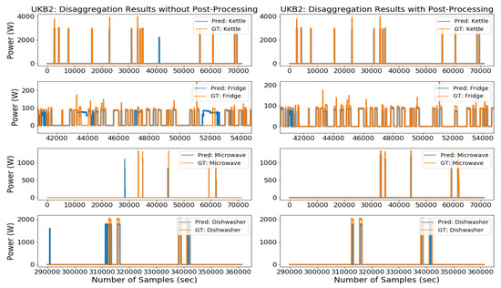
Figure 1. Seen Scenario—Disaggregation results of some target appliances from the UKDALE dataset with and without post-processing.
Table 1. Performance evaluation of the proposed algorithm in a seen scenario based on the UKDALE datasets.
| House # | Appliances | Without Post-Processing | With Post-Processing | ||||||
|---|---|---|---|---|---|---|---|---|---|
| F1 | MAE (W) | SAE | EA | F1 | MAE (W) | SAE | EA | ||
| 1 | Kettle | 0.658 | 2.162 | 0.179 | 0.911 | 0.995 | 1.837 | 0.217 | 0.891 |
| 1 | Fridge | 0.497 | 13.980 | 0.138 | 0.919 | 0.997 | 5.679 | 0.347 | 0.826 |
| 5 | Microwave | 0.535 | 65.090 | 0.028 | 0.986 | 0.719 | 21.450 | 0.515 | 0.743 |
| 2 | Dishwasher | 0.559 | 13.076 | 0.094 | 0.953 | 0.749 | 5.877 | 0.419 | 0.790 |
| 1 | Washing Machine | 0.322 | 65.720 | 1.010 | 0.492 | 0.795 | 18.870 | 0.655 | 0.673 |
| 2 | Electric Stove | 0.886 | 3.519 | 0.623 | 0.688 | 0.981 | 0.240 | 0.005 | 0.997 |
| 2 | Television | 0.976 | 0.976 | 0.018 | 0.991 | 0.995 | 0.497 | 0.012 | 0.994 |
| Overall | 0.633 | 23.503 | 0.298 | 0.848 | 0.890 | 7.778 | 0.310 | 0.845 | |
The disaggregation results of seven appliances are shown in Table 2. These results were calculated using 1-month data which was unseen during training. Not all the appliances were present in all six houses of the ECO dataset. Kettle, fridge, and washing machine data were obtained from house-1, whereas dishwasher, electric stove, and television data were retrieved from house-2 of the ECO dataset. Similarly, microwave data were obtained from house-5 of the ECO dataset. Type-2 appliances such as the dishwasher and washing machine are very hard to classify because of various operational cycles present during their operation. With our proposed MFS-LSTM integrated with post-processing, type-2 appliances have successfully been classified and their power consumption estimation resembles ground-truth consumption according to Figure 2.
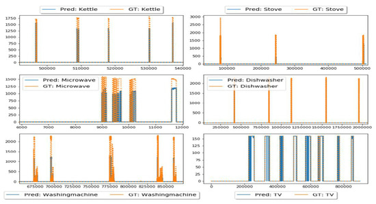
Figure 2. Seen Scenario: Disaggregation results of all target appliances from the ECO dataset
Table 2. Performance evaluation of the proposed algorithm in a seen scenario based on the ECO datasets.
| House # | Appliances | Without Post-Processing | With Post-Processing | ||||||
|---|---|---|---|---|---|---|---|---|---|
| F1 | MAE (W) | SAE | EA | F1 | MAE (W) | SAE | EA | ||
| 2 | Kettle | 0.961 | 3.906 | 0.004 | 0.998 | 0.981 | 2.353 | 0.043 | 0.978 |
| 2 | Fridge | 0.838 | 13.667 | 0.170 | 0.915 | 0.995 | 4.039 | 0.121 | 0.939 |
| 2 | Microwave | 0.721 | 7.285 | 0.276 | 0.862 | 0.869 | 5.402 | 0.437 | 0.781 |
| 2 | Dishwasher | 0.745 | 25.736 | 0.024 | 0.988 | 0.891 | 12.346 | 0.288 | 0.856 |
| 2 | Washing Machine | 0.189 | 30.990 | 0.686 | −0.09 | 0.701 | 5.400 | 0.641 | 0.679 |
| 2 | Rice Cooker | 0.299 | 8.900 | 0.699 | −0.161 | 0.781 | 1.115 | 0.378 | 0.811 |
| 5 | Electric Oven | 0.550 | 68.611 | 0.448 | 0.594 | 0.736 | 28.911 | 0.013 | 0.993 |
| 5 | Television | 0.512 | 5.695 | 0.219 | 0.890 | 0.879 | 3.428 | 0.649 | 0.675 |
| Overall | 0.688 | 23.541 | 0.361 | 0.714 | 0.976 | 8.999 | 0.367 | 0.959 | |
Although our algorithm was able to classify all target appliance activations, the presence of irrelevant activations in Figure 6 (left) indicates that the deep LSTM model learned some features of non-target appliances during training. This can happen due to the similar looking activation profiles of type-1 and type-2 appliances. This effect was eliminated with the use of the post-processing technique whose advantage can easily be realized with the results shown in Table 1 and Table 2 for a seen scenario.
The generalization capability of our network was tested using unseen data during training. Data used for testing the algorithms was completely unseen for the trained model. In this test case, we used entire house-5 data from the UKDALE dataset for disaggregation and made sure that the testing period contains activations from all target appliances. The UKDALE dataset contains 1-sec and 6-sec sampled mains and sub-metered data, therefore, we up-sampled ground truth data to 1-sec for comparison.
Performance evaluation results of the proposed algorithm with and without post-processing in the unseen scenario are presented in Table 3. In the unseen scenario, the post-processed MFS-LSTM algorithm achieved an overall F1-score of 0.746, which was 54% better than without post-processing. Similarly, MAE reduced from 26.90W to 10.33W, SAE reduced from 0.782 to 0.438, and estimation accuracy (EA) improved from 0.609 to 0.781 (28% improvement). When MAE, SAE, and EA scores of the unseen test case were compared with the seen scenario then a visible difference in overall results was observed. One obvious reason for this difference was the different power consumption patterns of house-5 appliances; also, %-NR was higher in house-5 (72%) as compared to the house-2 noise ratio, which was 19%. However, overall results prove that the proposed algorithm can estimate the power consumption of target appliances from the seen house but can also identify appliances from a completely unseen house with unseen appliance activations.
Table 3. Performance evaluation of the proposed algorithm in an unseen scenario based on the UKDALE dataset.
| House # | Appliances | Without Post-Processing | With Post-Processing | ||||||
|---|---|---|---|---|---|---|---|---|---|
| F1 | MAE (W) | SAE | EA | F1 | MAE (W) | SAE | EA | ||
| 5 | Kettle | 0.701 | 14.973 | 0.685 | 0.657 | 0.965 | 1.966 | 0.058 | 0.971 |
| 5 | Fridge | 0.732 | 27.863 | 0.270 | 0.865 | 0.872 | 19.608 | 0.467 | 0.766 |
| 5 | Microwave | 0.242 | 0.546 | 0.504 | 0.748 | 0.317 | 0.392 | 0.828 | 0.586 |
| 5 | Dishwasher | 0.554 | 35.129 | 0.273 | 0.863 | 0.809 | 15.275 | 0.323 | 0.838 |
| 5 | Washing Machine | 0.189 | 30.990 | 2.18 | −0.09 | 0.765 | 14.422 | 0.512 | 0.744 |
| Overall | 0.484 | 21.900 | 0.782 | 0.609 | 0.746 | 10.333 | 0.438 | 0.781 | |
Apart from individual appliance evaluation, it is also necessary to analyze total energy contributions from each target appliance. In this way, we can understand the overall performance of the algorithms when acting as a part of the NILM system. This information is helpful to analyze algorithm performance on estimating power consumption of composite appliances for a given period and how it is closely related to actual aggregated power consumption.
Figure 3 shows energy contributions from all target appliances in both seen and unseen test cases from the UKDALE and ECO datasets. The first thing to notice from Figure 3 is the amount of estimated power consumption, which is less than actual power consumption in both datasets. This happened because of the elimination of irrelevant activations which caused extra predicted energy. Another useful insight is the difference between the amount of estimated power consumption and actual consumption for type-2 appliances (dishwasher, washing machine, electric oven), which is relatively higher than the type-1 appliances difference. This could have happened due to multiple operational states of type-2 appliances which are very hard to identify as well as their power consumption is also very difficult to estimate by the DNN models. Energy contributions for all target appliances of the ECO dataset (Figure 1) are higher as compared to UKDALE appliances. This is due to the time span during which energy consumption by individual appliances was computed. For the UKDALE dataset, 1-week test data was used for evaluation. Whereas for the ECO dataset, one-month data was used for evaluation. Detailed results for energy consumption evaluation in terms of noise-ratio, percentage of disaggregated energy, and estimation accuracy are shown in Table 4.
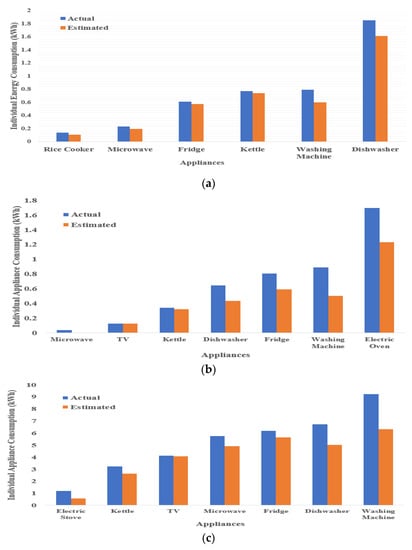
Figure 3. Energy contributions by individual appliances from (a) UKDALE House-2, (b) UKDALE House-5, (c) ECO House-1 and 2.
Table 4. Details of energy contributions by target appliances in UKDALE and ECO datasets.
| Metrics | UKDALE H-2 |
UKDALE H-5 |
ECO H-1 |
ECO H-2 |
|---|---|---|---|---|
| Noise Ratio (%) | 19.34 | 72.08 | 83.76 | 70.51 |
| Actual Disaggregated Energy (%) | 80.66 | 27.92 | 16.24 | 29.49 |
| Predicted Energy (%) | 63.15 | 21.57 | 12.99 | 24.53 |
| Estimation Accuracy | 0.891 | 0.886 | 0.900 | 0.916 |
As described in Section 3.3, the noise ratio refers to energy contribution by non-target appliances. In our test cases, total energy contributions by all target appliances in said houses were 80.66%, 27.92%, 16.24%, and 79.49% respectively. Based on the results presented in Table 4, our algorithm successfully estimated power consumption of target appliances with an accuracy of 0.891 in UKDALE house-2, 0.886 in UKDALE house-5, 0.900 for ECO house-1, and 0.916 for ECO house-2.
We compared the performance of our proposed MFS-LSTM algorithm with the neural-LSTM [1], denoising autoencoder (dAE) algorithm [2], CNN based sequence-to-sequence algorithm CNN(S-S) [3], and benchmark implementations of the factorial hidden Markov model (FHMM) algorithm, and the combinatorial optimization (CO) algorithm [4] from the NILM toolkit [5]. We chose these algorithms for comparison for various reasons. First, the neural LSTM, dAE, and CNN(S-S) were also evaluated on the UKDALE dataset. Secondly, these algorithms were validated on individual appliance models as we did. Thirdly, [1][2][3] also evaluated their approach on both seen and unseen scenarios. Lastly, recent NILM works [6][7][8] have used these algorithms (CNN(S-S), CNN(S-P), neural-LSTM) to compare their approaches. That is why these three are referred to as benchmark algorithms in the NILM research.
UKDALE house-2 and house-5 data were used to train and test benchmark algorithms for seen and unseen test cases. Four-month data was used for training, whereas 10-day data was used for testing. The min-max scaling method was used to normalize the input data and individual models of five appliances were prepared for comparison. Hardware and software specifications were the same as described in Section 3.2.
Table 5 shows training and testing times for the above-mentioned disaggregation algorithms in terms of length of days. Many factors affect the training time of algorithms, including training samples, trainable parameters, hyper-parameters, GPU power, and complexity of the algorithm. Considering these factors, the combinatorial optimization (CO) algorithm has the lowest complexity, thus it is the fastest to execute [9]. This can also be observed from the training time of the CO algorithm from Table 5. The FHMM algorithm was the second-fastest followed by the dAE algorithm. Training time results show that the proposed MFS-LSTM algorithm has faster execution time than the neural-LSTM and CNN(S-S) because of the fewer parameters and relatively simple deep RNN architecture.
Table 5. Computation time comparison between disaggregation algorithms (in seconds).
| Algorithms | Training (133 Days) |
Testing (10 Days) |
|---|---|---|
| CO | 11 | 1.00 |
| FHMM | 166 | 50.63 |
| dAE | 300 | 0.02 |
| Neural-LSTM | 1280 | 0.68 |
| CNN (S-S) | 1899 | 1.19 |
| MFS-LSTM | 908 | 0.65 |
Figure 4 shows the load disaggregation comparison of the MFS-LSTM with dAE, CNN(S-S), and neural-LSTM algorithms in the seen scenario. Qualitative comparison from Figure 4 shows that the MFS-LSTM algorithm disaggregated all target appliances and proved better as compared to the dAE, neural-LSTM, and CNN(S-S) algorithms in terms of power estimation and states estimation accuracy. Although, all algorithms correctly estimated operational states of target appliances. However, the dAE algorithm showed relatively poor power estimation performance for the disaggregating kettle, fridge, and microwave. The CNN(S-S) performance was better for the disaggregating microwave. However, for all other appliances, its performance seemed to be comparative with the MFS-LSTM algorithm. These findings can be better understood through quantitative scores for all algorithms in terms of the F1 score and estimation accuracy as shown in Table 6.
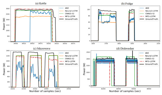
Figure 4. Comparison of disaggregation algorithms in the seen scenario based on the UKDALE dataset.
Table 6. Performance evaluation of disaggregation algorithms in the seen scenario.
| Performance Metrics | Algorithms | Kettle | Fridge | Microwave | Dishwasher | Washing Machine | Overall |
|---|---|---|---|---|---|---|---|
| F1 | CO | 0.291 | 0.493 | 0.322 | 0.125 | 0.067 | 0.259 |
| FHMM | 0.263 | 0.442 | 0.397 | 0.053 | 0.112 | 0.253 | |
| dAE | 0.641 | 0.735 | 0.786 | 0.746 | 0.485 | 0.679 | |
| Neural-LSTM | 0.961 | 0.791 | 0.774 | 0.419 | 0.152 | 0.619 | |
| CNN(S-S) | 0.940 | 0.912 | 0.923 | 0.708 | 0.759 | 0.848 | |
| MFS-LSTM | 0.981 | 0.995 | 0.869 | 0.891 | 0.701 | 0.887 | |
| MAE (Watts) | CO | 61.892 | 53.200 | 59.141 | 71.776 | 121.541 | 73.510 |
| FHMM | 84.270 | 67.244 | 53.472 | 107.655 | 147.330 | 91.994 | |
| dAE | 22.913 | 23.356 | 9.591 | 24.193 | 27.339 | 21.478 | |
| Neural-LSTM | 7.324 | 22.571 | 7.449 | 19.465 | 109.144 | 33.190 | |
| CNN(S-S) | 5.033 | 13.501 | 7.004 | 26.516 | 8.414 | 12.094 | |
| MFS-LSTM | 2.353 | 4.039 | 5.402 | 12.346 | 5.400 | 5.908 | |
| SAE | CO | 0.438 | 0.358 | 0.747 | 0.472 | 0.611 | 0.525 |
| FHMM | 0.463 | 0.516 | 0.849 | 0.594 | 0.523 | 0.589 | |
| dAE | 0.576 | 0.108 | 0.681 | 0.028 | 0.217 | 0.322 | |
| Neural-LSTM | 0.114 | 0.028 | 0.309 | 0.711 | 0.695 | 0.371 | |
| CNN(S-S) | 0.052 | 0.154 | 0.368 | 0.575 | 0.433 | 0.316 | |
| MFS-LSTM | 0.043 | 0.121 | 0.437 | 0.288 | 0.641 | 0.306 | |
| EA | CO | 0.926 | 0.915 | 0.838 | 0.581 | 0.847 | 0.821 |
| FHMM | 0.902 | 0.912 | 0.829 | 0.543 | 0.802 | 0.798 | |
| dAE | 0.711 | 0.946 | 0.659 | 0.986 | 0.723 | 0.805 | |
| Neural-LSTM | 0.943 | 0.940 | 0.845 | 0.645 | 0.614 | 0.797 | |
| CNN(S-S) | 0.972 | 0.930 | 0.717 | 0.723 | 0.745 | 0.817 | |
| MFS-LSTM | 0.978 | 0.939 | 0.781 | 0.856 | 0.679 | 0.847 |
As shown in Figure 4, the dAE’s F1 score was lower for the kettle as compared to all other algorithms. The neural-LSTM performed better in terms of the F1 score except for the dishwasher and washing machine. The CNN(S-S) performance remained comparative with the MFS-LSTM for all target appliances. The CO and FHMM algorithms showed lower state estimation accuracy compared to all other algorithms. When overall (average score) performance was considered, the MFS-LSTM achieved an overall F1 score of 0.887, which was 5% better than the CNN(S-S), 31% better than the dAE, and 43% better than the neural-LSTM and 200% better than the CO and FHMM algorithms. Considering the MAE scores, the MFS-LSTM achieved the lowest mean absolute error for all target appliances with an overall score of 5.908 watts. Only the CNN(S-S) scores were a bit close to the MFS-LSTM scores, however, the overall MAE score of the MSF-LSTM was two times less than CNN (S-S), almost four times less than the dAE, and six times less than the neural-LSTM.
Considering SAE scores, our algorithm achieved lowest SAE score of 0.043 for kettle, 0.121 for fridge, and 0.288 for dishwasher. MFS-LSTM algorithm’s consistent scores for all target appliances ensured an overall SAE score of 0.306, which was very competitive with CNN(S-S), Neural-LSTM and dAE. However, overall score of 0.306 was 71.6% lower than CO, and 92.5% lower than FHMM algorithm. When estimation accuracy scores were considered, then dAE power estimation accuracy was higher for fridge and dishwasher, and lower for microwave and washing machine. EA scores for Neural-LSTM algorithm were lower for multi-state appliances. However, MFS-LSTM algorithm achieved an overall estimation accuracy of 0.847 for being consistent in disaggregating all target appliances with high classification and power estimation accuracy.
Table 7 shows performance evaluation scores for benchmark algorithms in unseen scenario. F1, MAE, SAE, and estimation accuracy scores again proves effectiveness of MFS-LSTM algorithm in unseen scenario compared to benchmark algorithms. Considering F1 score, it can be observed that MFS-LSTM algorithm achieved more than 0.76 score for all target appliances except for microwave. MFS-LSTM achieved an overall score of 0.746, which was 200% better than Neural-LSTM, 27% better than CNN(S-S) and 22% better than dAE algorithm. MAE scores for MFS-LSTM were lower for all target appliances as compared to benchmark algorithms in unseen scenario. Our algorithm achieved an overall score of 10.33 watt, which was six times lower than dAE and CNN(S-S), and seven times lower than Neural-LSTM. Same trend was also observed with SAE scores, in which MFS-LSTM algorithm achieved lowest SAE scores for all target appliances except for microwave. An overall SAE score of 0.438 for MFS-LSTM algorithm was 38% lower than CNN(S-S), 59% lower than CO, 80% lower than FHMM and 87% lower than Neural-LSTM.
Table 7. Performance evaluation of disaggregation algorithms in the unseen scenario.
| Performance Metrics | Algorithms | Kettle | Fridge | Microwave | Dishwasher | Washing Machine | Overall |
|---|---|---|---|---|---|---|---|
| F1 | CO | 0.327 | 0.382 | 0.086 | 0.128 | 0.124 | 0.209 |
| FHMM | 0.181 | 0.539 | 0.022 | 0.047 | 0.101 | 0.178 | |
| dAE | 0.746 | 0.671 | 0.432 | 0.652 | 0.415 | 0.583 | |
| Neural-LSTM | 0.331 | 0.364 | 0.216 | 0.165 | 0.113 | 0.238 | |
| CNN(S-S) | 0.783 | 0.684 | 0.226 | 0.495 | 0.533 | 0.544 | |
| MFS-LSTM | 0.965 | 0.872 | 0.317 | 0.809 | 0.765 | 0.746 | |
| MAE (Watts) | CO | 113.457 | 89.922 | 77.264 | 81.131 | 77.902 | 87.935 |
| FHMM | 174.744 | 78.511 | 183.472 | 105.626 | 128.756 | 134.222 | |
| dAE | 64.864 | 56.785 | 19.283 | 164.931 | 23.958 | 65.964 | |
| Neural-LSTM | 89.514 | 58.562 | 14.841 | 106.390 | 103.654 | 74.592 | |
| CNN(S-S) | 54.244 | 23.675 | 21.191 | 113.447 | 115.783 | 65.668 | |
| MFS-LSTM | 1.966 | 19.608 | 0.392 | 15.275 | 14.422 | 10.333 | |
| SAE | CO | 0.813 | 0.374 | 0.951 | 0.625 | 0.715 | 0.696 |
| FHMM | 0.871 | 0.569 | 0.982 | 0.754 | 0.763 | 0.788 | |
| dAE | 0.581 | 0.552 | 0.867 | 2.112 | 0.585 | 0.939 | |
| Neural-LSTM | 1.588 | 0.573 | 0.815 | 0.505 | 0.614 | 0.819 | |
| CNN(S-S) | 0.523 | 0.624 | 0.843 | 0.339 | 0.691 | 0.604 | |
| MFS-LSTM | 0.058 | 0.467 | 0.828 | 0.323 | 0.512 | 0.438 | |
| EA | CO | 0.608 | 0.633 | 0.405 | 0.443 | 0.431 | 0.504 |
| FHMM | 0.589 | 0.551 | 0.336 | 0.417 | 0.584 | 0.495 | |
| dAE | 0.709 | 0.724 | 0.566 | −0.061 | 0.375 | 0.463 | |
| Neural-LSTM | 0.209 | 0.713 | 0.592 | 0.749 | 0.540 | 0.561 | |
| CNN(S-S) | 0.581 | 0.778 | 0.533 | 0.417 | 0.634 | 0.589 | |
| MFS-LSTM | 0.971 | 0.766 | 0.586 | 0.838 | 0.744 | 0.781 |
Estimation accuracy scores were also high for the MFS-LSTM with an overall score of 0.781. One noticeable factor is the difference in scores between the MFS-LSTM and all other algorithms in the unseen scenario. The differences shown prove the superiority of the proposed algorithm in the unseen scenario as well. Considering the noised aggregate power signal, our multi-feature input space-based approach together with post-processing can disaggregate target appliances with high power estimation accuracy as compared to state-of-the-art algorithms.
In accordance with Table 4 parameters, UKDALE house-2 and house-5 noise ratio was 19.34% and 72.08%, respectively. This implies that total predictable power was 80.66% and 27.92%. In order to estimate the percentage of predicted energy (energy contributions by all target appliances), estimation accuracy scores for all disaggregation algorithms are shown in Table 8. Presented results also highlight the proposed algorithm’s superior performance with an estimation accuracy of 0.994 and 0.956 in the seen and unseen test cases, respectively. These results suggest that our proposed algorithm efficiently estimates the power consumption of all target appliances for a given period of time.
Table 9. Evaluation of total energy contributions by target appliances in disaggregation algorithms.
| Algorithms | Estimation Accuracy (EA) | |
|---|---|---|
| Seen Scenario | Unseen Scenario | |
| CO | 0.907 | 0.544 |
| FHMM | 0.813 | 0.536 |
| dAE | 0.888 | 0.518 |
| Neural-LSTM | 0.891 | 0.289 |
| CNN (S-S) | 0.924 | 0.633 |
| MFS-LSTM | 0.964 | 0.856 |