1000/1000
Hot
Most Recent
 +1 point
Hydrological models are a simplified representation of the natural hydrological processes. These models are developed to understand processes, test hypothesis, and support water resources decision-making. However, as they are simplification of the natural processes, they are inherently uncertain. Their uncertainty primarily stems from their structure, parameter, input and calibration data observations. While parameter and structural uncertainties are related to both data information content and process conceptualizations, input and calibration data observations are a result of data information content. In order to enable an improved process understanding and better decision making, a systemic uncertainty analysis of all of the four sources is critical.
Hydrological models are developed to understand process, test hypothesis, and support decision-making. These models solve empirical and governing equations at different complexities. Their complexities vary depending on how the governing equations are solved over different spatial configurations such as lumped [1], semi-distributed [2], or fully distributed area [3], as well as the extent to which variables and processes are coupled [4][5]. Although model development has progressed in accounting for different processes and complexities, they remain as simplifications of the actual hydrological processes.
Process simplification is a consequence of limited knowledge and data, imprecise measurements, and involvement of multiple scales and interactive processes [6][7][8][9]. These simplifications introduce uncertainty and make it an intrinsic property of any model [10][11][12]. Analyzing this uncertainty requires separate methodological treatments beyond model development. However, uncertainty analysis (UA) benefits hydrological modeling in (i) identifying model limitations and improvement strategies [13][14], (ii) guiding further data collection [15][16], and (iii) quantifying the uncertainty associated with model predictions.
Various UA techniques have been developed. A few of the methods include generalized likelihood uncertainty estimation (GLUE) [17], differential evolution adaptive metropolis (DREAM) [18], parameter estimation code (PEST) [19], Bayesian total error analysis (BATEA) [20], and multi-objective analysis (Borg) [21]. These techniques have been applied in different water resources decision-making such as water supply design [22], flood mapping [23][24], and hydropower plant evaluation [25]. However, there is a lack of a systematic review and categorization of these techniques to provide a much-needed UA guideline for selecting a suitable method.
Hydrological model uncertainties stem from parameters, model structure, calibration (observation) and input data (Figure 1). In addition to these sources, uncertainties can stem from model initial and boundary conditions; however, these sources are not considered in this review. Hydrological models often contain parameterizations that are a result of conceptual simplifications, known as effective parameters [26]. Parameter uncertainty can be a result of the inability to estimate or measure these effective parameters that integrate and conceptualize processes [27]. In addition, parameter uncertainty can be a result of the natural process variability and observation errors. Although some model parameters, such as hydraulic conductivity, are measurable at the point scale, their values at the catchment scale vary significantly. Hence, the practical difficulty in measuring this variability can also lead to parameter uncertainty. On the other hand, due to errors in the calibration data, parameter uncertainty can be encountered even if a model is an exact representation of the hydrologic system. Therefore, inability to accurately estimate effective parameters, the challenge of measuring natural variability, and the existence of observation errors lead to parameter uncertainty. This uncertainty often manifests itself in model calibration through the lack of a single optimal set of parameters [28].
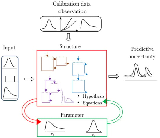
Figure 1. Different sources of hydrological model uncertainty. The arrows indicate the direction of interaction of the uncertainty sources. The center rectangle demonstrates different structures, hypotheses, and equations as examples of structural uncertainty. The top and left rectangles indicate input data distributions as sources of input forcing and calibration data uncertainties. The bottom rectangle shows parameter uncertainty using parameter distributions. The right-side sketch shows the resultant predictive uncertainty in a hydrograph as upper and lower predictive bands.
An exact representation of a hydrological system is challenging due to the absence of a unifying theory, limited knowledge and numerical and process simplifications. Such limitations constitute model structural uncertainty. Model structural uncertainty can also refer to alternative conceptualizations, such as the hydro-stratigraphy of the subsurface or the discretization of surface and process features [29][30][31]. Model performance is strongly dependent on model structures [32]. As a result, structural uncertainty is critical as it can render the model and quantification of other uncertainties useless [32][33][34]. Comparing structural and parameter uncertainty, Højberg et al. [35] showed that structural uncertainty is dominant, particularly when the model is used beyond its calibration sphere. Moreover, Rojas et al. [36] concluded that structural uncertainty may contribute up to 30% of the predictive uncertainty. Using the variance decomposition of streamflow estimates, Troin et al. [37] showed that model structure is the highest predictive uncertainty contributor.
Input forcing to hydrological models includes different hydro-meteorological, catchment, and subsurface data. Although there have been improvements in data acquisition and processing, the data used for model forcing are sparse, and subjected to gaps, imprecisions, and uncertainties [38]. In most cases, input data involve interpolations, scaling, and derivation from other measurements that result in an uncertainty range of 10–40% [38]. These inaccuracies in input data constitute input uncertainty. Failure to account for input uncertainty can lead to biased parameter estimation [20][39] and mislead water balance calculations [40]. Consequently, input uncertainty can interfere with the quantification of predictive uncertainty. Comparing input and model parameter uncertainty particularly in a data sparse region, Bárdossy et al. [41] showed the severity of input uncertainty over parameter uncertainty and suggested a simultaneous analysis of both uncertainties to have a meaningful result.
Hydrological modeling often involves calibrating the model parameters and evaluating model predictions using observed state and/or flux variables, such as streamflow and groundwater levels. These observations are subjected to similar measurement uncertainties as input data. Streamflow observations, for instance, are derived from rating curves that translate river stage measurements to discharge estimates. This translation not only propagates the random and systematic stage measurement errors but also passes the structural (rating curve equation) and parameter uncertainties involved in the calibration of the rating curve. In addition, discharge estimates suffer from interpolation and extrapolation errors of the rating curve, hysteresis, change in site conditions (e.g., bed movement), and seasonal variations in measurement and flow conditions [42][43][44][45]. Extrapolation contributes the highest uncertainty [46][47][48]. Overall, discharge observation uncertainty ranges from 5% [49][50] to 25% when extrapolation is involved [51].
Predictive uncertainty is the result of the above uncertainties exhibited on the model output. This uncertainty can be biased or variance-dominated depending on the level of model complexity and the information content of the data, bias being dominant in simple models and variance being dominant in complex models. Predictive uncertainty is usually heteroscedastic, the magnitude of uncertainty varying with the magnitude of the model output (non-Gaussian residuals). In streamflow modeling, this is partly due to the limited number of high flow observations (low frequency events) to constrain model calibration. Different data transformation schemes are used to address heteroscedasticity including the Box–Cox transformation and simple log transformation [47][48].
We have found six broad classes of UA methods: (i) Monte Carlo sampling, (ii) response surface-based schemes including polynomial chaos expansion and machine learning, (iii) multi-modeling approaches, (iv) Bayesian statistics, (v) multi-objective analysis, and (vi) least square-based inverse modeling (Figure 2). Furthermore, approximation and analytical solutions based on Taylor series are also used in UA. However, since such approaches are not widely applied, they are not included in this review.
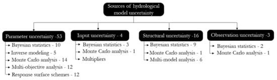
Figure 2. Summary of sources of hydrological model uncertainty and broad techniques used to deal with them.
The number of papers reviewed in this section across the different sources and methods are shown in Figure 2. This numbers indicate pioneering articles, articles that discuss limitations and advantages of the methods, and articles that introduce method improvements. Hence, the numbers do not indicate articles that are application oriented. As rainfall multipliers are embedded as part of model parameters they are not included as a unique method to be reviewed. In general, although it could be a limited sample, the numbers may reflect an approximation of how different methods are being developed for each source and how these methods are being critiqued and advanced as a focus of different studies.
The bellow six broad classes are a summary of different UA methods (Table 1). The common thread across these methods is their involvement of many actual/surrogate model executions. This can translate into high computational time depending on (1) the model’s execution time, (2) whether the surrogate training requires multiple runs, and (3) whether the model execution is parallel.
Table 1. Summary of uncertainty analysis methods, sources of uncertainty, and color coded broader methodological categories.
| No. | UA Methods Reviewed | Applicable in Uncertainty Source | Method Classes | Web Page to Download the Software Tool | Reference Application |
|---|---|---|---|---|---|
| 1 | Monte Carlo | Parameter/input/ structural uncertainty | Monte Carlo | http://www.uncertain-future.org.uk/?page_id=131 | [52] |
| 2 | GLUE | Parameter/ structural uncertainty | Monte Carlo and behavioral threshold | http://www.uncertain-future.org.uk/?page_id=131 | [53] |
| 3 | FUSE | Structural | Monte Carlo | https://github.com/cvitolo/fuse | [54] |
| 4 | Multi-objective | Parameter uncertainty | Multi-objective optimization | http://borgmoea.org/https://faculty.sites.uci.edu/jasper/software/; http://moeaframework.org/index.html |
[55][56][57] |
| 5 | Machine Learning | Predictive uncertainty | Machine Learning | https://scikit-learn.org/stable/ | [58] |
| 6 | PEST/UCODE | Parameter/ predictive uncertainty | Least square analysis | http://www.pesthomepage.org/ https://igwmc.mines.edu/ucode-2/ |
[59][60][61] |
| 7 | Polynomial chaos expansion | Predictive/ parameter uncertainty | Polynomial chaos expansion | https://www.uqlab.com/featureshttp://muq.mit.edu/ https://pypi.org/project/UQToolbox/ https://github.com/jonathf/chaospy |
[62][63][64] |
| 8 | Ensemble averaging | Structural uncertainty | Multi-models | [65] | |
| 9 | BMA | Structural uncertainty | Multi-models plus Bayesian statistics | https://faculty.sites.uci.edu/jasper/software | [66] |
| 10 | HME | Structural uncertainty | Multi-models plus Bayesian statistics | https://faculty.sites.uci.edu/jasper/software | [67] |
| 11 | DREAM | Parameter/input uncertainty | Bayesian statistics | https://faculty.sites.uci.edu/jasper/software/ | [18] |
| 12 | BATEA and IBUNE | Input/structure/ parameter uncertainty | Bayesian statistics | https://faculty.sites.uci.edu/jasper/software/ | [68][69] |
Compared to the other sources of uncertainty, several techniques are employed to address parameter uncertainty (Figure 2). One of the widely used parameter UA methods is generalized likelihood uncertainty estimation (GLUE) [17], which accounts for the equifinality hypothesis [28]. The equifinality hypothesis highlights the existence of multiple parameter sets that describe hydrological processes indiscriminately or producing the same final result. The approach augments Monte Carlo simulations with a behavioral threshold measure that distinguishes hydrologically tenable and untenable parameters (and structures). Although GLUE’s straightforward conceptualization and implementation allow it to achieve a widespread use, GLUE has been criticized for its subjectivity in choosing a behavioral threshold and its lack of a formal statistical foundation [70][71][72]. Extending GLUE, Beven [28] suggested the limits of acceptability approach where pre-defined uncertainties that objectively reflect both input and output observation uncertainties are used as a measure of acceptability than the subjective behavioral thresholds. Although its use is not as widespread as GLUE, this approach has been applied, e.g., [73][74]. The limitation of its application is partly due to the lack of measurements that reflect the level of input and output uncertainties and their interactions [75][76][77].
Following GLUE, numerous contributions have been made to formally quantify parameter uncertainty. These approaches primarily rely on Bayesian statistics [78][79][80][81]. The main advantage of the formal Bayesian statistics is that parameter uncertainty is not only quantified, but can also be reduced through the inclusion of prior knowledge. Although GLUE’s behavioral thresholds can achieve this goal, their formulation is subjective. The latest addition to the formal approach is DREAM [18], which has been applied widely. DREAM’s widespread application is derived from its unique capability of merging the differential evolution algorithm [82] with the adaptive Markov Chain Monte Carlo (MCMC) approach [83][84]. The differential evolution allows DREAM to efficiently explore non-linear and discontinuous parameter spaces, while the adaptive MCMC component keeps it within the parameter posterior space. Contrary to other MCMC schemes [85], DREAM uses multiple chains to exchange sampling space information rather than confirming the attainment of the stationary state. The primary challenge of DREAM and other Bayesian methods is identifying a likelihood function that results in homoscedastic residuals, justifying the use of a strong assumption for a formal likelihood function. This challenge is particularly difficult in disproportionately low flow dominated observations of streamflow coupled with a few high flows [28][47][86][87][88].
Least squares-based parameter inversions incorporated in PEST [19] and US Geological Survey computer program (UCODE) [61] are also used to quantify parameter uncertainty. These approaches rely on linear approximation of models and Gaussian residuals. Besides estimating parameter uncertainty, these methods are also useful in determining the number of model parameters that can be estimated using the available data [89][90]. This is valuable in highly parameterized models to prioritize data collection for model improvement. Furthermore, PEST expedites Monte Carlo based UA through its null space Monte Carlo analysis and the use of singular value decomposition (SVD). This further allows PEST to be used in its SVD-assist mode with Tikhonov regularization. The SVD-assist approach coupled with parallelized Jacobian matrix calculation makes parameter estimation close to observations (because of Tikhonov regularization) and faster (due to parallelization plus SVD reducing the parameter space) when calibrating highly parameterized and ill-posed problems. The main limitations of PEST and other least-squared based UA are their assumption of model linearity and Gaussian residuals. These assumptions have limited their use in surface water models riddled with threshold-based processes, discontinuities and integer variables.
Multi-objective optimization (MOO) is another UA approach for parameter uncertainty. MOO-based UA has received substantial interest due to the absence of a single global optimal solution due to equifinality, and because of the need for improved constraint of flux and store outputs in hydrological models [55][91][92]. MOO allows retrieving information from the increasingly available data against which model predictions can be compared [56][93]. It handles parameter uncertainty by conditioning model calibration through multiple complementary and competing objective functions. The functions can be defined using (1) multiple responses such as, metrics that measure the matching of different segments of a hydrograph, (2) same-variable output but at multiple sites, and (3) multi-variable outputs such as streamflow, soil moisture, and evapotranspiration [56][94][95]. The result of MOO provides trade-off solutions referred to as non-dominated (Pareto) solutions in which each member solution matches some aspect of the objective better than every other member.
Parameter uncertainty is considered well identified when the optimized parameter uncertainty substantially decreased from the prior uncertainty, leading to a reduced model prediction uncertainty. In MOO, the uncertainty range can further be narrowed by rejecting solutions that failed the model validation test. MOO also provides unique parameter uncertainty information following the shape of the Pareto front. For instance, extended Pareto front in each objective indicates high uncertainty in reproducing the parameterization of the processes [56][95][96]. Furthermore, MOO provides functionality beyond parameter UA as the shape of the tradeoff allows us to understand model structural limitations [97]. However, this advantage might not be straightforward because meaningful multi-objective tradeoffs in hydrological modeling are less frequent [97].
One of the challenges in MOO is the lack of consistent criteria for choosing the number and type of the objective functions and inability to formally emphasize one criterion over the other. Like GLUE, MOO is also statistically informal as it does not use Bayesian probability theory. Theoretically, the Pareto solutions and GLUE’s behavioral solutions may overlap; however, they are not necessarily equivalent. The difference between the parameter uncertainty sets defined by the Pareto front and the GLUE approach is that GLUE’s equifinality set consists of both the dominated and non-dominated parameter whereas the Pareto set contains only the non-dominated sets [98]. The difference between Bayesian UA and multi-objective analysis is that Bayesian schemes usually have a single objective (likelihood functions) or an aggregated multi-objective. In cases where multi-objective configuration is employed, the Bayesian scheme results in a compromise solution [99] while MOO results in a full Pareto solution [98]. Detailed review of MOO can be found in [95].
Response surface methods are used to approximate predictive uncertainty that is primarily caused by parameter uncertainty. Response surface methods employ a proxy function emulating the original model’s parameter and output relationships, making the method blind to model internal workings or the nature of outputs that are not emulated. The common proxy functions used to approximate models are truncated Polynomial Chaos Expansion (PCE) [2][100][101] and machine learning schemes [102][103][104][105]. Since these methodologies are computationally inexpensive, the approximation is suited for UA in complex models that demand long run time or applied for real time forecasts. Response surface methods train the approximating functions based on a subset of the original model output and parameter relationships. Consequently, one of the major challenges of these schemes is ensuring the accuracy of the approximating function. If the subset is not representative, the function can lead to biased approximation. Identifying the right size and representative subset are an ongoing research. Furthermore, the accuracy of the response surface methods depends on the smoothness of the original model parameter and output surface relationship. Thus, the approximation is better for problems that are not highly non-linear and response surfaces that are not riddled with thresholds and multiple local optimums. Commonly, a validation test on a split sample is considered to confirm the approximating function’s accuracy [2][105].
The typical approach of uncertainty quantification using response surfaces is to conduct Monte Carlo simulations using the approximated function. The resultant Monte Carlo based distributions represent the predictive uncertainty. Compared to the machine learning alternative, PCE offers an analytical approximation of the uncertainty through the estimate of variance without the need for simulations [106]. Further review of PCE can be found in [107][108], while review of machine learning approaches are provided by [109].
Dotto et al. [110] compared Monte Carlo (GLUE), multi-objective (A Multi-Algorithm, Genetically Adaptive Multiobjective—AMALGAM [57]) and Bayesian (Model-Independent Markov Chain Monte Carlo Analysis—MICA [111]) techniques to estimate parameter uncertainty. They found that while all the techniques performed similarly; GLUE was slow but easiest to implement. Although the Bayesian technique was less suitable because it required homoscedastic residuals, it was the only one avoiding subjectivity. Finally, they indicated that method choice depends on the modelers’ experience, priority, and problem complexity. Further, Keating et al. [112] found equivalent performance between the Bayesian DREAM and the least square null-space Monte Carlo. Comparing GLUE and formal Bayesian techniques, Thi et al. [113] indicated formal Bayesian method’s efficiency in resulting to a better identified parameter. However, Jin et al. [114] indicated that a stricter behavioral threshold choice can achieve similar identifiability with an increased computation [115]. A detailed comparison of formal Bayesian techniques against GLUE and its behavioral threshold choices can be found in [115].
Hydrological models require different hydroclimatic input data. For this review, we focused on precipitation and its uncertainty. Traditionally, input uncertainty is addressed using a factor that multiplies input precipitation to correct measurement uncertainty. This approach is relatively fast and easy as the multiplication factor is expert judgement-based or estimated with model parameters. However, the method is ad hoc and does not have formal procedures to determine the multiplying factor. Beyond this approach, precipitation uncertainties can be studied using Monte Carlo (GLUE) and Bayesian statistics. The Monte Carlo approach estimates the rainfall multiplying along with the model parameters. The Bayesian techniques can be classified into two classes, model dependent and model independent, depending on whether the input uncertainty is estimated dependently or independently of the model parameters. Balin et al. [116] demonstrated how input uncertainty can be estimated as a standalone quantity, separate from model parameters. They decoupled input uncertainty from the model by assuming a distribution that represents the “true” precipitation. This approach is advantageous, because it relieves input uncertainty from the remaining uncertainty sources. However, the approach is limited because of the difficulty in determining the “true” input distribution.
On the other hand, Bayesian total error analysis (BATEA [69]) and integrated Bayesian uncertainty estimator (IBUNE [68]) estimate input uncertainty along with model parameters. Hence, these approaches recover input uncertainty with parameter and structural uncertainties. Thereby, the estimated input uncertainty is dependent on the specific model structure and can vary with changes in model structures. Consequently, the input uncertainty might not only be a result of input measurements, but also structural and parameter uncertainties. These approaches can also be computationally expensive in distributed models, which require spatially and temporally varying inputs.
Multi-model averaging and ensemble techniques, which pool together alternative model structures, have been applied to quantify and reduce structural uncertainty. Hagedorn et al. [117] noted that the success of multi-model averaging is a result of error compensation, consistency, and reliability. Consistency refers to the lack of a single model that performs best regardless of circumstances, and reliability refers to averages performing better than the worst component an ensemble. Moreover, Moges et al. [118] showed why a multi-model average performs better than a single model using statistical proof and empirical large-sample data.
Predictions from ensembles are combined using either equal or performance-based weights. Velázquez et al. [65] presented a study that benefits from equal weighting while performance based weighted multi-model predictions are discussed in [32][66][119]. A comparison of different alternative model averaging techniques was presented in [120]. Equal weighting is advantageous in the absence of model weighting/discrimination criteria and when component models have similar performances. However, when the models’ performances are significantly different and each model is specialized in simulating certain components of the hydrological processes, using variable weights provide better predictions.
One of the widely used weighted multi-model averaging is Bayesian model averaging (BMA) [121][122][123]. BMA and similar Bayesian based averaging techniques are advantageous since their weights are interpretable and derived from model posterior performance that combines the model’s ability to fit observations and experts’ prior knowledge. Despite its widespread application, BMA has its limitations in addressing structural uncertainty. For instance, even though model performance varies across hydrograph segments [124], runoff seasons [14], or catchment circumstances [67], BMA assigns constant weights to component models. Furthermore, improvement in BMA’s performance was noted when component models are weighted differently for different quantiles of a hydrograph [124]. In contrast, hierarchical mixture of experts (HME) [67], an extension of BMA, has the capacity to assign different weights to different models depending on the dominant processes governing different segments of a hydrograph. This flexibility allows HME to be useful in dealing with structural uncertainty when model performances vary.
Hydrology involves governing physical principles and established process signatures that need to be respected. As a result, any statistically based multi-model averaging techniques need to be critically streamlined so that they respect hydrological principles. In this regard, Gupta et al. [125] stressed the application of diagnostic modeling. Similarly, Sivapalan et al. [126] argued the importance of parsimony and incorporation of dominant processes in model structural development. To this end, Moges et al. [127] streamlined HME by coupling it with hydrological signatures that diagnose model inadequacy. Such approaches can be explored to characterize catchment hydrology while avoiding disparities between statistical success and process description.
Structural uncertainty has also been addressed in the framework for understanding structural errors (FUSE [54]), which explores structural uncertainty through shuffling and combination of parts of alternative hydrological models. The parts constitute alternative formulations of processes. FUSE has similarity with Monte Carlo (or Bootstrap) methods. However, the samples in FUSE are components of a model representing the different alternative process conceptualizations. Further, given the ease of parallelization, FUSE is practical to address structural uncertainty.
The chief criticism of all multi-modeling UA is the limitation of identifying and incorporating the entire span of feasible model structures. Although the above methods can handle any number of structures, the practical inability to identify and explore the entire structural space constrains the scope of the investigation. As a result, full examination of structural uncertainty is limited.
Although different calibration data are used to constrain hydrological models, streamflow observation uncertainty is common in the literature. Hence, this subsection focuses on streamflow observation uncertainty. Some of the methodologies used to address observation uncertainty include Monte Carlo simulations to estimate the rating curve uncertainty, use of the upper and lower bounds of the rating curve estimates, and Bayesian techniques. The first method propagates observation uncertainty to parameter and/or predictive uncertainty estimates through a repeated calibration of the hydrologic model [40], making the method computationally intensive. In the second approach, only the upper and lower rating curve uncertainty bounds are considered to come up with the corresponding upper and lower bounds of predictive uncertainty [128]. This approach is computationally effective, but it does not maximize exploring the full information contained in the rating curve uncertainty. To improve the rating curve uncertainty utilization, McMillan et al. [129] suggested derivation of an informal likelihood function that accounts for the entire rating curve uncertainty. This technique allowed them to apply Bayesian statistics and use the rating curve information to analyze observation uncertainty. In contrast, Sirakosa and Renard [130] used a formal Bayesian technique where the rating curve parameters and the hydrological model parameters are inferred simultaneously by directly using the stage measurement instead of the streamflow estimate.
Observation uncertainty influences predictive uncertainty. McMillan et al. [129] showed improvement in model predictive uncertainty by considering discharge observation uncertainty compared to a model that does not consider discharge uncertainty while Beven and Smith [77] demonstrated the disinformation emanating from observation uncertainties. Aronica et al. [128] showed how different rating curve realizations lead to different predictive uncertainties, whereas Engeland et al. [40] concluded that considering or not considering observation uncertainty leads to different parameter uncertainties and different interactions with structure, parameter, and predictive uncertainties. These studies indicate the significance of observation uncertainty and the need to account it.
The resultant uncertainty estimate of a model output is predictive uncertainty. Predictive uncertainty can be quantified by propagating parameter, structure and input uncertainties to the model output. This propagation is mostly performed by Monte Carlo simulation of parameter, structure, and input uncertainties. Predictive uncertainty can be reduced using different machine learning schemes [58][131]. Although their physical process realism needs validation, these schemes reduce predictive uncertainty as they can learn and identify patterns in the model residuals. Besides, to reduce predictive uncertainty, it is important to disentangle and understand the propagation of the different sources of uncertainties.