1000/1000
Hot
Most Recent
 +1 point
Turbulent flow can be numerically resolved with different levels of accuracy. Many numerical approaches for solving turbulence have been proposed, such as the Reynolds-Averaged Navier–Stokes (RANS), the Large Eddy Simulation (LES), and Direct Numerical Simulation (DNS) approaches. Among these numerical methods, the RANS approach, specifically the Eddy Viscosity Model (EVM), is widely used for calculating turbulent flows thanks to its relatively high accuracy in predicting the mean flow features and its more limited computational demands. However, this approach suffers from several weaknesses, e.g., compromised accuracy and uncertainties due to assumptions in the model construction and insufficient incorporation of the fluid physics. In the LES approach, the whole eddy range is separated into two parts, namely, the large-scale eddy and subgrid-scale (SGS) eddy. The former can be directly resolved, while the latter is computed using the SGS model. As the computing power rapidly increases, this approach is extensively used to study turbulence physics and to resolve low-to-medium Reynolds number flows.
In the RANS approach, instantaneous solution variables in the governing equations are decomposed into the mean and fluctuating components, as expressed in Equation (1).
Substituting this variable expression into the instantaneous continuity and Navier-Stokes (N-S) equations yields the ensemble- or time-averaged forms for single-phase Newtonian flow, as shown in Equations (2) and (3). Henceforth, repeated-suffix summation convention is used in the formulae.
The fluctuating quantities are included in the Reynolds stress tensor (−ρu′iu′j¯¯¯¯¯¯) with six components. In order to close the equation set, the Reynolds stress tensor needs to be appropriately solved. One of the solutions for this closure problem employs the Boussinesq assumption [1], which relates the Reynolds stresses to the mean velocity gradients. The advantage of the Boussinesq assumption is the relatively low computational cost due to its simplicity. This works well for the engineering flows, which are dominated by only one turbulent shear stress such as the jet flow, wall boundary layer flow, and mixing layers flow. However, this approach is insensitive to the streamline curvature, rotation and body forces, and it exhibits a poor performance in the flows with a strong anisotropy or stress transport effect [2][3]. It also has difficulty in predicting transitional flows.
It is worth noting that the turbulent viscosity used in solving the Reynolds stress terms is a function of the space and flow features, rather than a physical parameter such as the fluid viscosity, which is dependent on the molecular structure of the fluid. Obviously, the turbulent viscosity needs to be solved before computing the Reynolds stress terms. In this paper, two-equation models, which include two additional transport equations, are reviewed. Usually the turbulence kinetic energy (k) is adopted as one equation and the turbulent kinetic energy dissipation rate (ε) or the specific dissipation rate (ω) as another one. The modified versions of the ε/ω model will also be presented here. Due to length restrictions, the zero- and one-equation models are not included in the article, but they may be found elsewhere [4][5][6].
The standard k-ε (SKE) model was originally proposed by Launder and Spalding [7]. The model has been widely applied for resolving turbulent flows without a severe pressure gradient or strong swirling effect (e.g., plane jet, mixing layer, and boundary layer flows) because of its relatively high robustness, low computational cost, and reasonable accuracy. Equations (4) and (5) show the general form of k and ε. By solving these two transport equations, the turbulent viscosity can be calculated as expressed in Equation (6).
The terms from left to right in Equations (6) and (7) are the respective local time derivative, convection, diffusion, production, sink, and source terms. The SKE model is derived from a fully turbulent flow with high Reynolds numbers. The viscous effect is ignored in the model. However, this cannot be applied in the vicinity of the wall, where the viscous force dominates the flow characteristics. In order to deal with this problem, either a wall function is adopted with the SKE model, or a low Reynolds number model is used. The former confuses the users’ judgement whether the weakness of this method lies in the basic SKE model itself or in the wall function. The latter requires additional functions to modify the standard transport equations. With respect to the low Reynolds number models [8][9][10][11][12][13][14], an example proposed by Lam and Bremhorst (LB model) [13] is presented in Equations (7) and (8).
where:
Compared with the SKE model, different formulations of functions f1, f2 and fμ are developed in the LB model to describe the near-wall behavior better. It has been confirmed that the function fμ has a predominant influence on the model performance, and functions f1, f2 play a secondary role in the performance [15].
There are also other modified versions of the SKE model, amongst which the widely used Renormalization Group (RNG) k-ε model [16] and the Realizable k-ε (RKE) model [17] are introduced in the following section. The main differences between the RNG k-ε model and the SKE model are the modifications of the turbulent viscosity and ε sink term. A differential equation is analytically derived for effective viscosity μeff to account for the low Reynolds number effect. This feature can improve the predictive ability of the RNG k-ε model for low Reynolds number flows or near-wall flows. Additionally, a new ε destruction term is used to account for the rapid strain by modifying the constant of this term. The RKE model is modified mainly with regard to the turbulent viscosity and the ε equation. By defining a variable Cμ [17][18][19] instead of a constant value in turbulent viscosity formulation, the RKE model satisfies the realizability constraints, i.e., positive values for the normal stresses and the Schwartz inequality for the shear stresses. In order to increase the robustness of the model, a new ε equation is employed based on a dynamic equation for fluctuating vorticity. The new ε equation describes turbulent vortex stretching and turbulent dissipation more appropriately compared to the ε equation in the SKE model. With the modified ε equation, the well-known round-jet anomaly that is a poor prediction of the spreading rate of round/axisymmetric jet may be solved [17].
The k-ω model is widely used for turbulence modelling [20]. Different versions of this model have been developed in the last decades [21][22][23][24][25][26][27]. In this paper, the most well-known k-ω model proposed by Wilcox [21] is reviewed. The transport equations of this model are presented in Equations (10) and (11), where the calculation of β1 refers to the work of Wilcox [21].
Unlike the k-ε model, the k-ω model can be integrated through the viscous sublayer without any damping function to account for the low Reynolds number effect with high numerical stability. Therefore, it is well applied in aerodynamic flows [22][20]. However, the k-ω model is highly sensitive to the empirical value of ω at the free edge of the turbulent shear layer, which can lead to a large prediction error. In order to solve this problem, a modified model was proposed with combination of the original k-ω model and the SKE model by adding a blending function [22]. This new model is termed the Baseline k-ω model, which applies the original k-ω model in the near-wall region and switches to the SKE model in the outer region. The Baseline k-ω model has a similar performance to the original k-ω model in boundary layer flows, but the former one avoids the strong freestream dependence. However, both k-ω models fail to predict the onset and amount of separation in adverse pressure gradient flows. Based on the Baseline k-ω model, further modification to eddy viscosity is proposed to account for the transport effects of the principal turbulent shear stress, leading to a significant improvement in predicting the adverse pressure gradient flows [22]. However, the introduced blending function depends on empiricism (e.g., the distance to wall), limiting its application to flows in complex geometries.
All the aforementioned methods belong to the category of the Eddy Viscosity Model (EVM). Some other advanced EVMs were developed [28][29][30][31][32]. In order to account for the strong anisotropy in the near-wall region, Durbin [28] adopted a new turbulent viscosity term defined in Equation (12), which is considered to be more appropriate than that defined in Equation (6) in a near-wall region. A separate transport equation for a wall-normal turbulent stress υ2¯¯¯ was proposed and solved with the aid of the elliptic relaxation concept. This model is termed the υ2-f model, where f represents the elliptic relaxation function. Subsequently, several modified versions were proposed with respect to the velocity scale [31], the characteristic length [29], the function f [32], and the variable υ2¯¯¯ [30]. This model category performs well for pressure-induced separating flow, buoyancy impairing turbulent flow, and backstep flow [31][32][33].
where:
In addition to the modified versions of the linear EVM, the idea of non-linear EVM has been substantially used [34][35][36][37][38][39][40]. Even though these modified models demonstrated certain improvements over linear EVMs in predicting flows with a strong streamline curvature or turbulent stresses in the near-wall sublayer, they are still inferior to the more advanced model, e.g.
In order to overcome the limitations of the EVM, Second-Moment Closure (SMC) models abandoning the Boussinesq assumption have been developed. The SMC model directly solves the transport equation for each of the Reynolds stress terms. Since the SMC approach considers the effects of streamline curvature, rotation, and rapid change of strain rate in a more rigorous manner, it is long expected to replace the currently widely applied two-equation models. The SMC model class consists of the Algebraic Stress Model (ASM) and the Differential Stress Model (DSM). ASM is derived from differential stress transport equations by invoking the weak-equilibrium assumption [41][42][43]. It ignores the transport terms of the anisotropy by assuming that the transport of the Reynolds stress is proportional to that of turbulent kinetic energy [44][45]. In general, the ASM is considered an intermediate tool between the LEVM and the DSM. Due to the space limitation, only the DSM is presented in this paper. A symbolic representation of the stress transport equation is expressed in Equation (14). In addition, a scale-determining equation, i.e., the ε equation, is needed to complete the DSM.
The terms from left to right represent the local time derivative of Reynolds stress, convection, turbulent diffusion, molecular diffusion, stress production, buoyancy production, pressure strain, dissipation and source, respectively. The sij term is user-defined for a specific stress transport source. If there is no source, this term becomes zero. It is required to model DT,ij, Gij, ϕij and εij to close the equation, while it is not necessary to model Lij, Cij, DL,ij and Pij.
The DT,ij term includes the velocity transport and the pressure transport. The velocity triple moments can be measured, whereas the pressure transport is intractable. Usually, the pressure transport is considered to be negligible [46]. Therefore, the model is mainly designed for the velocity triple moments. The most popular model is the generalized gradient-diffusion model proposed by Daly and Harlow (DH) [47]. The DH model has a symmetry problem in the indices, leading to dependence on the coordinate frame. Subsequently, some variants of this model were developed by Hanjalic and Launder [48], Shir [49], Mellor and Herring [50]. More complex models were also put forward by Nagano and Tagawa [51] and Magnaudet [52]. Due to uncertainties in the modelling equations, the complex models may not necessarily outperform the simplified models. Given more computing resources consumed by the complex models and a poor convergence, application of these models in engineering has been doubted [53][54].
Compared to the εij and Gij terms, it is necessary to pay extra attention to model ϕij. Usually, the ϕij term is decomposed into three parts, namely, the slow pressure-strain term ϕij,1, rapid pressure-strain term ϕij,2, and wall-reflection term ϕij,w. Not all of the models introduced below include the third term. Rotta [55] proposed a linear model for ϕij,1, which considers that ϕij,1 is proportional to the stress anisotropy tensor. However, this linear model is unable to satisfy the realizability constraints. A general quadratic model [56] is proposed to solve this problem. Linear [48][57][58][59] and nonlinear models [60][61][62] were proposed to model the ϕij,2 term. Even though the nonlinear model is considered to be theoretically advanced, the complexity of the formulation prohibits its application for engineering computation. The turbulence anisotropy is enhanced due to the damping effect of the normal stress by the wall. This damping affects both the pressure-strain terms. In order to account for the damping effect, a commonly used model [49][63] is presented to model the wall-reflection term ϕij,w. However, this model involves a variable, i.e., the normal distance to the wall. This is believed to be a major weakness. For purpose of overcoming this weakness, the elliptic relaxation concept and elliptic-blending method were proposed to account for the near-wall inhomogeneity, and more information on that can be found in [64][65].
The DSM is the most elaborate model in the RANS approach, which has an indisputable superiority over the rudimentary two-equation models in predicting complex flows, e.g., highly swirling and rotating flow, separating flow, and secondary flow. However, its application is limited by (1) a high degree of uncertainty in modelling the high-order correlation terms (e.g., pressure-strain and dissipative correlation) due to an insufficient knowledge of physics; (2) a high demand for computational resource (approximately 50–150% more computing time than a two-equation EVM [2]). Fortunately, due to the use of more advanced models (e.g., the DNS), the accuracy and robustness of the DSM have been improved. A rapid development in computer science (e.g., parallel processing and improved performance) satisfies the high computational need for the use of DSM model. The DSM has received more attention recently because of the failure of the EVM in predicting complex turbulent flows.
Turbulent flow features a wide range of eddy scales from the Kolmogorov length scale to the size comparable to the characteristic length of the mean flow. The large eddies contain most of the turbulent energy and are mainly responsible for the momentum and energy transfer. They are strongly affected by boundary conditions. The small eddies tend to be more isotropic and homogeneous, and their dissipation process is linked to fluid viscosity. For this reason, it is very difficult for the RANS approach to model all the eddies in a single model. The LES approach separates the large eddies from the small ones by employing a spatial filtering method [66] for the instantaneous governing equations. After that, the large eddies are directly resolved by the filtered equation, and the small ones (i.e., the Subgrid-Scale (SGS) eddies) are modelled by the SGS model. The filtered variable (donated by an overbar) is defined by Equation (15). The resulting continuity and momentum equations are expressed in Equations (16) and (17), showing similar forms but a different physical meaning for those in the RANS approach.
where σij refers to the stress tensor due to molecular viscosity, and τij represents the SGS stress term. Most of current SGS models adopt the Boussinesq assumption (termed the Eddy-Viscosity model), which relates the SGS stress to the large-scale strain-rate tensor, as shown in Equation (18). Based on the definition of the eddy viscosity, various SGS models [67][68][69][70][71] have been proposed. Smagorinsky [67] developed the first SGS model by assuming a local energy equilibrium between the large scale and the subgrid scale. The eddy viscosity in this model is defined in Equation (20). This model becomes very popular to date due to its simplicity, numerical robustness, and stability. However, it has several drawbacks: (1) the model constant varies with different flows; (2) the model cannot predict the inverse energy transfer (i.e., backscatter) due to its purely dissipative nature; (3) the model has difficulty in reproducing the correct mean quantities (e.g., SGS dissipation) as the grid scale approaches the integral scale; (4) the model does not yield a zero eddy viscosity in near-wall regions.
where:
In Equation (20), where:
where Δ represents the local grid scale. In order to solve the model constant problem, a Dynamic Smagorinsky–Lilly (DSL) model was proposed [68][69], where the model constant is dynamically calculated by using the resolved eddies with the scale size between the grid filter and test filter. The main advantage of this model is that it is not necessary to prescribe and/or tune the model constant. However, the DSL model is subjected to a numerical instability and a variable model constant. Germano [68] proposed an averaging method to overcome this weakness. A good performance was achieved in a channel flow simulation [72]. Another variant of Smagorinsky–Lilly model is the Dynamic Kinetic Energy (DKE) model [73][74][75]. Unlike the algebraic form in Smagorinsky–Lilly and DSL models, the DKE model solves an additional transport equation for the SGS turbulent kinetic energy instead of adopting the local equilibrium assumption. This model can better account for the energy transfer from the large-scale eddy at the cost of computational expenses. Some other variants of the Smagorinsky–Lilly model were formulated to solve the low Reynolds number effect in the near-wall region, one of which was based on the square of the velocity gradient tensor named the Wall-Adapting Local Eddy-viscosity (WALE) model [70]. Compared to the original Smagorinsky–Lilly model, the WALE model can produce a zero eddy viscosity in the vicinity of the wall or in a pure shear flow. Hence, this model does not need a damping function. In addition to the WALE model, a hybrid model [76] was proposed by combining the Smagorinsky–Lilly model with a damping function [77] to improve the predictive capability for wall-bounded flows. This hybrid model demonstrated a good performance in plane channel flow with different Reynolds numbers. However, this model involves a variable, i.e., the wall normal distance. The determination of this wall normal distance requires an empirical approach for specific flow.
In the framework of the eddy-viscosity SGS model, there are several alternatives to the Smagorinsky-type SGS model, such as Vreman’s model [78], the QR model [79][80], the σ-model [81], and the S3PQR model [82]. Compared to the Smagorinsky-type SGS model, Vreman’s model can predict zero eddy viscosity in near-wall regions or in transitional flows without explicit filtering, averaging or clipping procedures. However, it was found that the model coefficient in Vreman’s model is far from universal. To solve this problem, two procedures were proposed to dynamically determine the model coefficient, i.e., the one based on the global equilibrium between the subgrid-scale dissipation and the viscous dissipation [83][84] and the other one based on the Germano identity [85]. It was reported that the latter is better suited for transient flows [85]. The QR model, which is a minimum-dissipation eddy-viscosity model, gives the minimum eddy dissipation required to dissipate the energy of sub-filter scales. The advantages of this model lie in appropriately switching off for laminar and transitional flows, the low computational complexity, and consistency with the exact sub-filter tensor on isotropic grids. The disadvantage of this model is the insufficient eddy dissipation, which can be corrected by increasing the model constant. Moreover, the QR model requires an approximation of the filter width to be consistent with the exact sub-filter tensor on anisotropic grids. It was noted that the accuracy of the model result for anisotropic grids is highly dependent on the used filter width approximation. By modifying the Poincaré inequality used in the QR model, the dependence can be removed, leading to the construction of an anisotropic minimum-dissipation model that generalizes the desirable properties of the QR model to anisotropic grids [86]. For the purpose of meeting a set of properties based on the practical/physical considerations, the σ-model based on the singular values of the velocity gradient tensor was developed [81]. Owing to its unique properties, ease of implementation, and low computational cost, the σ-model is considered to be suitable for complex flow configurations. Subsequently, through comparison between static and dynamic σ-models, it was found that the local dynamic procedure is not suited for the σ-model, and a global dynamic procedure is suggested [87]. Trias et al. [82] built a general framework for LES eddy-viscosity models, which is based on the 5D phase space of invariants. By imposing appropriate restrictions in this space, a new eddy-viscosity model, i.e., the S3PQR model, was developed. In addition to meeting a set of desirable properties such as positiveness, locality, Galilean invariance, proper near-wall behavior, and automatic switch-off for laminar, 2D and axisymmetric flows, this new model is well-conditioned and has a low computational cost, with no intrinsic limitations for statistically inhomogeneous flows. Despite of all the merits of this model, special attention should be given to the calculation of the characteristic length scale and the determination of the model constant before engineering applications.
Alternatives to the eddy-viscosity SGS model are the similarity model [88][89][90][91], the velocity estimation model [92][93], the Approximate Deconvolution model (ADM) [94][95][96], and the regularization model [97][98][99]. The similarity model class adopts the idea that an accurate approximation for a SGS model can be reconstructed from the information contained in the resolved field. Therefore, the similarity models [88][89][90][91] approximate the SGS stress tensor by a stress tensor calculated from the resolved scales. Due to this nature, the similarity model can naturally account for the inverse energy transfer (i.e., backscatter). This is different from the eddy viscosity model, which only considers the global SGS dissipation (i.e., the net energy flux from the resolved scales to the subgrid scales). It is worth mentioning that, due to the importance of accurate prediction of the inverse energy transfer, a dynamic two-component SGS model was proposed to include the non-local and local interactions between the resolved scales and subgrid scales [91]. The model correctly predicted the breakdown of the net transfer into forward and inverse contributions in a priori tests. In some cases, however, the similarity model underestimated the SGS dissipation. An extra dissipative term was added to solve this issue. This new model formulated is also referred to as the mixed model. Furthermore, the similarity model and the mixed model need additional computational resources due to the implementation of the second filtering. Special attention should be paid to choose an appropriate filter type and size. Following the same idea, Domaradzki et al. [92] improved the SGS stress approximation by replacing the unknown unfiltered variables by approximately deconvolved filtered variables. Subsequently, this SGS model based on the estimation of the unfiltered velocity, which was originally formulated in spectral space, was extended to the physical space [93]. It was found that both versions of this velocity estimation model perform better than or are comparable to classical eddy viscosity models for most physical quantities. This model can account for backscatter without any adverse effects on the numerical stability. Several questions for improving the model need to be addressed, such as the modelling of nonequilibrium and high Reynolds number turbulence in three Cartesian directions. Stolz et al. [94][95][96] proposed a formulation of the ADM for LES, in which an approximation of the unfiltered solution is obtained from the filtered solution by a series expansion involving repeated filtering. Given a good approximation of the unfiltered solution at a time instant, the nonlinear flux terms of the filtered N-S equations can be computed directly, avoiding the explicit computation of the SGS closures. The effect of the non–represented scales is modelled by a relaxation regularization involving a second filtering and a dynamically estimated relaxation parameter. The ADM is evaluated for incompressible wall-bounded flow [95] and compressible flows [94][96]. The results showed that the ADM can have a significant improvement over the standard and dynamic Smagorinsky models, while at less computational cost compared with that of the dynamic models or the velocity estimation model. The high-Reynolds-number supersonic flow [100] and transitional flow [101] were investigated by the ADM. Agreement was observed between the ADM and experiments or DNS. For the former flow, a rescaling and recycling method was used to have a better control on the desired inflow data. Recently, the ADM was extended for a two-phase flow simulation [102]. By comparing the macroscopic flow characteristics, the ADM showed a better performance than the conventional LES model. However, further investigations should be performed on the relaxation term model for a two-phase simulation and microscopic characteristics of the dispersed phase in a 3D simulation. Another important class of the SGS model is the regularization model, which combines a regularization principle with an explicit filter and its inversion. The regularization model includes many versions, such as the Leray model [97], the Leray-α model [98][103], the Clark-α model [99], the Navier–Stokes-α (NS-α) model [104], etc. For the last one, several variants are proposed, including the NS-α deconvolution model [105][106][107][108] and the reduced order NS-α model [109][110]. It was found that the NS-α deconvolution model can significantly improve the prediction accuracy by carefully choosing the filtering radius and by correctly selecting the approximate deconvolution order [108]. Given the difficulties in efficient and stable simulation of the NS-α model for incompressible flows on coarse grids, the reduced order NS-α model is introduced by using deconvolution as an approximation to the filter inverse, reducing the fourth-order NS-α formulation to a second-order model. In spite of the success of the reduced order NS-α model, future work needs to be conducted on locally and dynamically choosing α and numerical testing on different benchmark flows, to name but a few. In addition, comparative studies have been performed between different regularization models [111][112][113], in which the capability of the regularization model has been demonstrated for a specific flow.
The LES is considered a compromise between the RANS and the DNS. It is more accurate than the RANS and it needs less computational resources than the DNS. However, the LES model has not reached the maturity stage as a numerical tool for the design or the parametric study of complex engineering flows, due to not only a high computational requirement, but also many unresolved issues such as ill-defined boundary conditions, wall-resolved flow, turbulent flow with chemical reactions, and compressible flow. Nevertheless, the LES model has been successfully applied in transitional flow [114][115][116][117], separated flow [118][119], and bubbly flow [120][121]. Figure 1 shows the calculation results in a separated boundary layer transition on a flat plate with a semi-circular leading edge of radius of 5 mm under elevated free-stream turbulence. A periodic boundary condition was adopted in the spanwise direction. Free-slip and no-slip conditions were used at lateral boundaries and the plate surface, respectively. The simulation agrees well with experimental data on mean and fluctuating streamwise velocities for an Enhanced-Turbulence-Level (ETL) case, demonstrating a good performance of the LES model for the transitional flow. Figure 2 shows a comparison between a modified k-ε model and the LES model in a bubbly flow. Compared with the experimental data, the LES model is superior in predicting the turbulence.
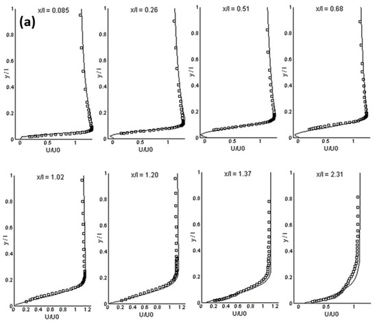
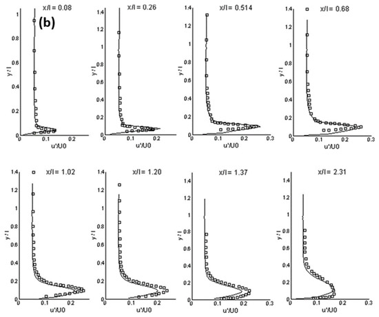
Figure 1. (a) Mean streamwise velocity, (b) rms streamwise velocity at different streamwise stations (ETL-case) (LES: solid lines, experimental data: symbols, x/l: normalized streamwise, y/l: wall-normal direction, U/U0: normalized mean streamwise velocity, u’/U0: normalized rms streamwise velocity) [117].
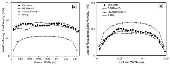
Figure 2. Comparison of model predictions with experimental data for (a) axial and (b) lateral liquid velocity fluctuations at a height of 0.25 m in a square cross-sectioned bubble column with a superficial gas velocity of 4.9 × 10⁻³ m/s [120].
The fluid behavior in the domain is largely determined by the inflow condition [122]. The treatment of the inflow condition is of significant importance for LES modelling. Currently, there are two main categories for generating the inflow data, namely, precursor simulation and a synthetic method. The former involves a separate simulation, where the periodic boundary condition or the recycling method can be used. The flow data are stored at each time step in this simulation and then introduced to the inlet boundary for modelling the flow of interest. The main advantage of this method is to obtain more realistic inflow conditions, which represent the required flow characteristics (e.g., velocity profile, turbulence intensity, shear stress, power spectrum, and turbulent structures). The inlet boundary, however, needs to be placed in an equilibrium region for scaling arguments in the precursor simulation, which may even not exist in some flows. This method may lead to a spurious periodicity for the time series [123]. In addition, running a separate simulation requires high computational costs especially for a high-Reynolds number flow. This restrains its application to complex engineering flows. The limitation can be reduced by an internal mapping method. This method integrates the precursor simulation into the main domain, mapping the data downstream of the inlet back to the inlet boundary [124][125].
The synthetic method as an alternative to the precursor simulation is expected to construct the inflow conditions for practical flows. The simplest way is to impose a white-noise random component on the inlet velocity. The magnitude of this random component is determined by the turbulent intensity. Since the turbulence-like component is rapidly dissipated due to the lack of spatial and temporal correlation, this white-noise method is inappropriate to generate the inflow data [126]. In order to impose realistic inflow data on the inlet boundary, other advanced synthetic methods have been developed. These advanced methods consist of the Fourier technique [127][128], principal orthogonal decomposition (POD) method [129][130], digital filtering technique [131][132], and synthetic eddy method (SEM) [133][134][135]. Several comparative studies have been performed on different synthetic methods [134][135][136][137]. Jarrin et al. [134] used the SEM in the hybrid RANS/LES simulations for turbulent flows from simple channel and square duct flows to the flow over an airfoil trailing edge. Compared to other synthetic methods (i.e., Batten’s method (Fourier method) [127] and random method), the SEM can substantially reduce the inlet section, leading to a large decrease in the CPU time. Figure 3 shows a better performance of the SEM in the inlet velocity vector compared to that of the others. The SEM realistically reproduced the magnitude and length scale of the fluctuations. The fluctuations in the Batten’s model decorrelated in space in the near-wall region due to the decomposition in Fourier’s mode. Recently, Skillen et al. [135] improved the SEM of Jarrin et al. (Original SEM) [133] with respect to the normalization algorithm and the eddy placement. The former leads to an improvement over the original SEM model. The latter saves a cost of around 1–2 orders of magnitude. Figure 4 and Figure 5 show the turbulent shear stresses and skin-friction coefficients from the original SEM [133], the improved SEM of Skillen et al. [135], and the precursor LES of Kaltenbach et al. [138]. In comparison with the original SEM, the improved SEM shows a better agreement with the precursor LES results both for the turbulent shear stress and the skin-friction coefficient. Although there is a rapid development of synthetic methods, the available synthetic methods are limited to construct the inflow condition with all required turbulence characteristics mentioned above. Further development is needed. It is unnecessary to claim which method is the best; however, the most appropriate method can be selected by considering the accuracy and the computational cost.
Figure 3. Velocity vectors of the LES inlet condition for hybrid simulation of channel flow: (a) precursor LES, (b) SEM, (c) Batten’s method, (d) random method (y/δ: normalized y distance, z/δ: normalized z distance, δ: initial boundary layer thickness) [134].
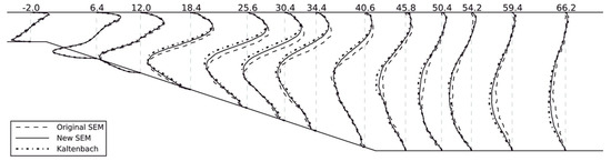
Figure 4. Profiles of turbulent shear stress (the number at the top of the figure indicates profile locations (the distance from the start of the incline, normalized by the initial boundary layer thickness)) [135].
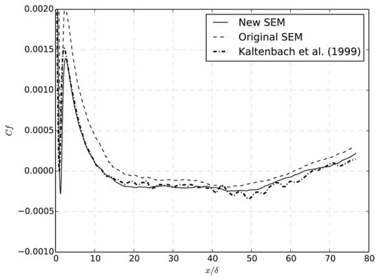
Figure 5. Wall shear stress for the inclined wall (Cf: wall shear stress, x/δ: normalized distance from the start of the incline) [135].