Application of CMAQ during SOAS

Version	Summary	Created by	Modification	Content Size	Created at	Operation
1		Petros Vasilakos	+ 2192 word(s)	2192	2021-06-10 11:00:25	\|
2	update references and layout	Amina Yu	Meta information modification	2192	2021-06-29 08:26:08	\| \|
3	update references	Amina Yu	Meta information modification	2192	2021-06-29 08:26:36	\|

This entry is adapted from the peer-reviewed paper 10.3390/atmos12060707

Formation of aerosol from biogenic hydrocarbons relies heavily on anthropogenic emissions since they control the availability of species such as sulfate and nitrate, and through them, aerosol acidity (pH). To elucidate the role that acidity and emissions play in regulating Secondary Organic Aerosol (SOA), we utilize the 2013 Southern Oxidant and Aerosol Study (SOAS) dataset to enhance the extensive mechanism of isoprene epoxydiol (IEPOX)-mediated SOA formation implemented in the Community Multiscale Air Quality (CMAQ) model (Pye et al., 2013), which was then used to investigate the impact of potential future emission controls on IEPOX OA.

IEPOX SOA Henry’s Law aerosol pH acidity emissions reductions non-volatile cations sensitivity

1. Ozone, NOx and Sulfate

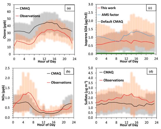
In all simulations including the base scenario, there was good agreement between the measurements and the simulated values of atmospherically relevant compounds at the Centreville site. Ozone was strongly correlated with the measurements, but exhibits a consistent positive bias of approximately 10 ppb (Figure 1a), while NO_x was captured well, albeit with less variability than the measurements (Figure 1b). Reasons for positive biases in model simulations of ozone in the SE US have been explored in Travis et al. 2016 ^[1] and could include but are not limited to errors in vertical mixing and production rates within the planetary boundary layer height (PBL). For aerosol species, sulfate closely tracked the measurements (Figure 1d), but was 26% lower during the middle of the day. Although there was an appreciable amount of isoprene OA predicted for the SE US, for the SOAS site IEPOX OA was much lower than the amount estimated from the Positive Matrix Factorization (PMF) factors derived from the measurements by almost 1.2 μg m⁻³. All of the above species, except for IEPOX OA, changed little with the modifications discussed below, while for the optimal H simulation it was about 30% lower than the PMF factor for SOAS ^[2] (Figure 2c). The initial simulation, where only semivolatile isoprene OA could form (default version of CMAQ without IEPOX extended chemistry), produced very little OA (Figure 2c—green line), indicating that semivolatile OA was only a small fraction of total isoprene OA.

Figure 1. Diurnal profiles during the Southern Oxidant and Aerosol Study (SOAS) campaign for measured (red), simulated (black) and default CMAQ (green) for (a) ozone, (b) NO_x, (c) isoprene SOA and (d) sulfate. The shaded areas represent one standard deviation at each diurnal hour. The default CMAQ 5.0.2, which includes only semivolatile isoprene OA (green) leads to very little isoprene SOA in (c).

1.2. Henry’s Law Sensitivity Tests and Updates to the Simulations

1.2.1. Baseline Simulation

Our initial simulation (hereafter baseline) used the default version of CMAQ as described in Pye et al. 2013. For this case, the Henry’s law coefficient for IEPOX was set to 2.7 × 10⁶ M atm⁻¹. Biogenic emissions for isoprene were not changed and left to the value generated by BEIS. The deposition surrogate used to calculate the dry deposition of IEPOX was methylhydroxyperoxide (CMAQ species VD_OP), with a relatively low H of 3.1 × 10² M atm⁻¹. The PBL was calculated by the WRF meteorology and used as is.

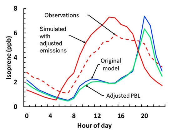
Results from the baseline simulation showed that IEPOX OA was severely underestimated, especially methyltetrols (MT) and organosulfates (OS). Isoprene levels were biased low during the day time and exhibited a night time high, suggesting that the isoprene emissions from BEIS were not accurate (Figure 3). However, IEPOX levels were overestimated when compared to the observations by a factor of 10. The relative ratios of IEPOX-derived OA (OS to MT) compared favorably with the observations, suggesting that the aqueous chemical mechanism represents the underlying physics accurately. Similarly, important gas phase and aerosol species, such as ozone, NO_x and sulfate were accurately predicted on average, although with some bias, possibly due to the long simulation period. To alleviate the issues identified with the simulation, we applied a number of sequential updates to the model by making use of the available measurements, in order to ensure that the gas phase products were as close as possible to the observed values before attempting any changes in the aqueous chemistry.

Figure 2. Observed (dashed-red), default model (blue), adjusted planetary boundary layer height (PBL, green) and adjusted PBL and emissions (solid red) isoprene diurnal profiles for the Centreville gridcell. Concentrations at each hour correspond to the campaign average for that hour.

1.2.2. Planetary Boundary Layer Height (PBL) Prescription and Isoprene Emission Fitting (IEF)

In order to rectify the unrealistic isoprene profile, the first change we applied to the model was direct the assimilation of PBL data available from SOAS, by replacing the model-predicted values with the measured ones. The PBL height predicted from WRF was biased high during the day and biased low during the night compared to observations, which is a known issue with WRF ^[3] that could explain the isoprene daytime low and its nighttime high. Results from the PBL simulation indicated that this change had little impact on all important tracers. Daytime isoprene levels remained similar to the baseline simulation, while there was a slight decrease of the nighttime high by 1 ppb (Figure 2). The PBL simulation indicated that the behavior of the isoprene levels was driven by the emissions and not by the meteorology, corroborated by simulated temperature profiles that closely matched the observed profiles.

Isoprene emissions in our simulations were under-predicted during the day time and overestimated during the night time, which led to the spike in isoprene concentration during the night (Figure 2). To resolve the issue, the measured isoprene emissions as well as the emissions predicted by BEIS were used, in order to determine scaling factors with which modelled isoprene emissions were multiplied at each model timestep as to better match the observed and simulated levels. As an initial guess the ratio of the measured to simulated values was used, which was then optimized through multiple linear regressions, to achieve better agreement between model and measurements. This simulation (referred to as isoprene emissions flux, or IEF) significantly improved isoprene levels and eliminated the daytime low and the nighttime high (Figure 3).

1.2.3. Isoprene Epoxydiol (IEPOX) Deposition Correction (DEP)

While the IEF simulation improved isoprene levels, the extreme overestimation of IEPOX still remained. Dry deposition for IEPOX is expected to be a significant loss process, given the stickiness of the molecule and propensity to deposit to wet surfaces ^[4]; however, the deposition surrogate used in CMAQ was methylhydroxyperoxide, a slowly depositing molecule, which has a Henry’s law constant four orders of magnitude less than that of IEPOX, meaning that depositional loss of IEPOX to wet surfaces was most likely significantly underestimated (depositional time scale of τ = 11 h). By changing the surrogate to HNO₃ in the deposition-adjusted (DEP) update, the timescale was reduced by 50% and there was a marked decrease of IEPOX levels to half of what they originally were. Surprisingly, IEPOX OA levels were not impacted by this change, suggesting that other processes were rate-controlling with regards to SOA production.

1.2.4. Updated IEPOX Gas Phase Oxidation and Henry’s Law Sensitivity Tests

After both the IEF and DEP changes, the IEPOX levels were still positively biased when compared to observations. A potential reason could be the underestimation of the gas phase IEPOX oxidation loss to OH. The rate constant used for the gas phase loss of IEPOX for the previous simulations was 1.5 × 10⁻¹ cm³ molecules⁻¹ s⁻¹ ^[4]. 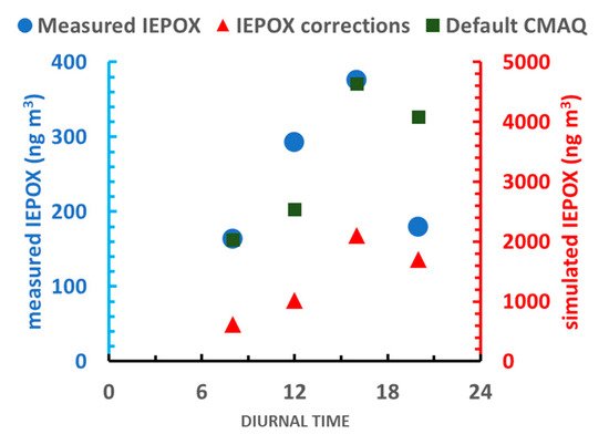We updated the rate constant for the gas phase loss of IEPOX to OH, to a value of 3.6 × 10⁻¹¹ cm³ molecules⁻¹ s⁻¹ ^[5]. The updated oxidation simulation, slightly reduced IEPOX levels by 5%, while keeping IEPOX OA levels approximately constant. The IEPOX overestimation remained (Figure 4) which implies that the existing sinks are still not significant enough or there is another removal process (for example an additional gas phase reaction) which is not included in the model.

After the above changes, and ensuring that there is sufficient gas phase IEPOX available to react in the aqueous phase, the negative bias for IEPOX OA persisted and the linear relationship between sulfate and IEPOX OA was still not captured ^[2]. The IEPOX Henry’s law constant is one of the most uncertain parameters of the system ^[6] and at the same time one the most important ones, since it directly controls the amount of IEPOX that is available in the aqueous phase to produce SOA. 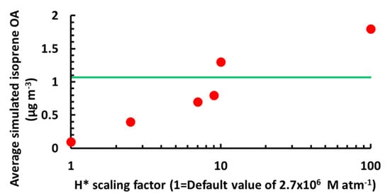The literature reported range for the Henry’s law constant for IEPOX spans more than 2 orders of magnitude ^[7]^[6]^[8], so a number of sensitivity tests were performed to estimate a value led to the most consistent results between the model and measurements, using as a constraint the correlation between sulfate and IEPOX OA from Xu et al. (2015), since it is a better indicator for the accuracy of the chemical processes included in the model than the concentration of IEPOX OA. We observed an almost linear relationship between the average levels of isoprene OA and the logarithm of H (Figure 4). A value of 1.9 × 10⁷ M atm⁻¹, which is similar to recent estimates, yields the best overall agreement ^[9]^[10]^[11]. A comprehensive list of simulated scenarios is shown in Table 1.

Figure 3. Measured (cyan), default CMAQ (green) and corrected (red) IEPOX diurnal concentrations. The IEPOX corrections data refers to IEPOX levels after updating both the deposition surrogate and the reaction rate constant for the OH⁻ reaction. Measurements from ^[12].

Figure 4. Isoprene organic aerosol (OA) sensitivity to H⁺ from the Henry’s law sensitivity tests. The horizontal axis is in units of 2.7 × 10⁶ M atm⁻¹, which corresponds to the default H value in Table 2013. CMAQ version. The green line denotes the average observed isoprene OA.

Table 1. List of simulated scenarios and their specifications. The Henry’s law coefficient H is equal to 2.7 × 10⁶ M atm⁻¹.

Simulation Name	PBL Height	Isoprene Emissions	IEPOX Deposition Surrogate	IEPOX + OH⁻ Oxidation Constant	H* Scaling Factor
BASELINE	default	default	VD_OP	Paulot	1
PBL	assimilated	default	VD_OP	Paulot	1
IEF	assimilated	adjusted	VD_OP	Paulot	1
DEP	assimilated	adjusted	HNO3	Paulot	1
Oxidation	assimilated	adjusted	HNO3	Jacobs	1
Henry 1	assimilated	adjusted	HNO3	Jacobs	2.5
Henry 2	assimilated	adjusted	HNO3	Jacobs	5
Henry 3	assimilated	adjusted	HNO3	Jacobs	7
Henry 4	assimilated	adjusted	HNO3	Jacobs	9
Henry 5	assimilated	adjusted	HNO3	Jacobs	10
Henry 6	assimilated	adjusted	HNO3	Jacobs	100

2. Comparing Aqueous SOA to Observations and Correlation with Sulfate

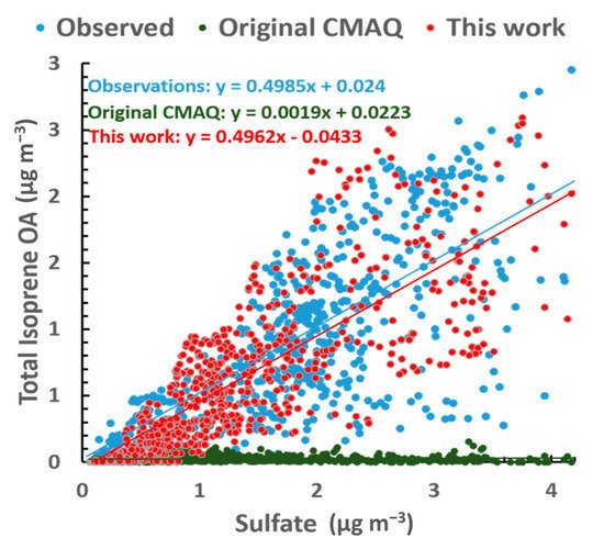
Recent studies ^[2]^[9]^[13] have observed a strong correlation between sulfate and isoprene OA in the vicinity of the SE US. To test the validity of the isoprene OA production mechanism in the current version of CMAQ, we used the coefficients of this linear relationship (slope and intercept) as the main parameters to be optimized with our Henry’s law sensitivity tests. The slope and intercept of the correlation were less susceptible to emission/model biases, since they were process controlled parameters (reaction and diffusion of IEPOX in the aqueous phase) and not governed by concentrations.

In the base case, without any updated or extended isoprene chemistry, there was a correlation between sulfate and isoprene OA; however, the levels of isoprene OA were far too low and the slope almost 0 (Figure 6). Using an H of 1.9 × 10⁷ M atm⁻¹, the simulated and observed correlations achieve remarkable agreement.

Figure 5. Correlation between sulfate and isoprene OA for the SOAS observations (blue), base scenario without updated chemistry (green) and optimal H simulation (red).

The other two important parameters which have been found to control the formation of isoprene OA are acidity (H⁺) and particle water (H₂O_ptcl) ^[2]^[9]^[14]^[15]. However, for the case of the SE US, only weak correlations between isoprene OA and H⁺ or H₂O_ptcl have been observed ^[2]^[9]. In other areas where aerosol pH is higher and water is less abundant, the predicted correlation could be much higher. Note that, for the needs of this analysis and, in the analysis presented in Xu et al. 2015, the definition of acidity used here uses only water as a solvent, which is consistent with recent studies ^[16] when assuming single-phase chemistry.

There is an abundance of aerosol water in the SE while, at the same time, the mean aerosol pH in Centreville is close to 1 indicating high H⁺ availability ^[17]^[18]. As such, the weak correlation can be explained since, due to their relative abundance, aerosol water and H⁺ do not constitute limiting parameters for the formation of IEPOX OA, and small changes in their value do not affect isoprene OA levels.

Another possible explanation for the strong correlation with sulfate and the weak correlation with H⁺ and H₂O_ptcl, is the competition between acidity and particle water, since increased levels of particle water lead to dilution of ions and reduced pH. In addition, the dilution could weaken a potential salting-in effect, suppressing the IEPOX uptake from the gas phase. While our model does not include this salting-in effect that could be important in some cases, by enhancing the solubility of IEPOX in the aqueous phase, it is not expected to have a strong effect in this study due to the large amounts of water present in the aerosol and the subsequent dilute concentrations of salt ions.

We observe similar behavior in the model when we perform multivariate linear regression on our results, indicating that the current version of the model is able to correctly capture the chemistry behind IEPOX OA production. The regression coefficients are provided in Table 2.

Table 2. Results for multiple linear regression of IEPOX OA with respect to sulfate, particle water and H⁺.

Regression Variable	Regression Coefficient in the Measurements (Xu et al. 2015)	Regression Coefficient for the Simulations
Sulfate	0.424	0.527
Water	−0.004	0.029
H⁺	0.009	0.007

References

Travis, K.R.; Jacob, D.J.; Fisher, J.A.; Kim, P.S.; Marais, E.A.; Zhu, L.; Yu, K.; Miller, C.C.; Yantosca, R.M.; Sulprizio, M.P.; et al. Why do models overestimate surface ozone in the Southeast United States? Atmos. Chem. Phys. 2016, 16, 13561–13577.
Xu, L.; Guo, H.; Boyd, C.; Klein, M.; Bougiatioti, A.; Cerully, K.; Hite, J.; Isaacman-VanWertz, G.; Kreisberg, N.M.; Knote, C.; et al. Effects of anthropogenic emissions on aerosol formation from isoprene and monoterpenes in the southeastern United States. Proc. Natl. Acad. Sci. USA 2014, 112, 37–42.
Hu, X.-M.; Klein, P.M.; Xue, M. Evaluation of the updated YSU planetary boundary layer scheme within WRF for wind resource and air quality assessments. J. Geophys. Res. Atmos. 2013, 118, 10490–10505.
Paulot, F.; Crounse, J.D.; Kjaergaard, H.G.; Kurten, A.; St Clair, J.M.; Seinfeld, J.H.; Wennberg, P.O. Unexpected epoxide formation in the gas-phase photooxidation of isoprene. Science 2009, 325, 730–733.
Jacobs, M.I.; Darer, A.I.; Matthew, J. Elrod Rate Constants and Products of the OH Reaction with Isoprene-Derived Epoxides. Environ. Sci. Technol. 2013, 47, 12868–12876.
Eddingsaas, N.C.; VanderVelde, D.G.; Wennberg, P.O. Kinetics and products of the acid-catalyzed ring-opening of atmospherically relevant butyl epoxy alcohols. J. Phys. Chem. A 2010, 114, 8106–8113.
Pye, H.O.T.; Pinder, R.W.; Piletic, I.R.; Xie, Y.; Capps, S.L.; Lin, Y.-H.S.; Surratt, J.D.; Zhang, Z.; Gold, A.; Luecken, D.J.; et al. Epoxide Pathways Improve Model Predictions of Isoprene Markers and Reveal Key Role of Acidity in Aerosol Formation. Environ. Sci. Technol. 2013, 47, 11056–11064.
Wang, C.; Yuan, T.; Wood, S.A.; Goss, K.-U.; Li, J.; Ying, Q.; Wania, F. Uncertain Henry’s law constants compromise equilibrium partitioning calculations of atmospheric oxidation products. Atmos. Chem. Phys. 2017, 17, 7529–7540.
Budisulistiorini, S.H.; Li, X.; Bairai, S.T.; Renfro, J.; Liu, Y.; Liu, Y.J.; McKinney, K.A.; Martin, S.T.; McNeill, V.F.; Pye, H.O.T.; et al. Examining the effects of anthropogenic emissions on isoprene-derived secondary organic aerosol formation during the 2013 Southern Oxidant and Aerosol Study (SOAS) at the Look Rock, Tennessee ground site. Atmos. Chem. Phys. 2015, 15, 8871–8888.
Nguyen, T.B.; Coggon, M.M.; Bates, K.H.; Zhang, X.; Schwantes, R.H.; Schilling, K.A.; Loza, C.L.; Flagan, R.C.; Wennberg, P.O.; Seinfeld, J.H. Organic aerosol formation from the reactive uptake of isoprene epoxydiols (IEPOX) onto non-acidified inorganic seeds. Atmos. Chem. Phys. 2014, 14, 3497–3510.
Chan, M.N.; Surratt, J.D.; Claeys, M.; Edgerton, E.S.; Tanner, R.L.; Shaw, S.L.; Zheng, M.; Knipping, E.M.; Eddingsaas, N.C.; Wennberg, P.O.; et al. Characterization and quantification of isoprene-derived epoxydiols in ambient aerosol in the southeastern United States. Environ. Sci. Technol. 2010, 44, 4590–4596.
Earth System Research Laboratory Chemical Sciences Division. Available online: (accessed on 31 May 2021).
Budisulistiorini, S.H.; Nenes, A.; Carlton, A.G.; McNeill, V.F.; Pye, H.O.; Surratt, J.D. Simulating Aqueous-Phase Isoprene-Epoxydiol (IEPOX) Secondary Organic Aerosol Production During the 2013 Southern Oxidant and Aerosol Study (SOAS). Environ. Sci. Technol. 2017, 51, 5026–5034.
Nguyen, T.; Petters, M.; Suda, S.; Guo, H.; Weber, R.; Carlton, A. Trends in particle-phase liquid water during the Southern Oxidant and Aerosol Study. Atmos. Chem. Phys. 2014, 14, 10911–10930.
Surratt, J.D.; Chan, A.W.H.; Eddingsaas, N.C.; Chan, M.N.; Loza, C.L.; Kwan, A.J.; Hersey, S.P.; Flagan, R.C.; Wennberg, P.O.; Seinfeld, J.H. Reactive Intermediates Revealed in Secondary Organic Aerosol Formation from Isoprene. Proc. Natl. Acad. Sci. USA 2010, 107, 6640–6645.
Schmedding, R.; Rasool, Q.Z.; Zhang, Y.; Pye, H.O.T.; Zhang, H.; Chen, Y.; Surratt, J.D.; Lopez-Hilfiker, F.D.; Thornton, J.A.; Goldstein, A.H.; et al. Predicting secondary organic aerosol phase state and viscosity and its effect on multiphase chemistry in a regional-scale air quality model. Atmos. Chem. Phys. 2020, 20, 8201–8225.
Guo, H.; Xu, L.; Bougiatioti, A.; Cerully, K.M.; Capps, S.L.; Hite, J.J.R.; Carlton, A.G.; Lee, S.-H.; Bergin, M.H.; Ng, N.L.; et al. Fine-particle water and pH in the southeastern United States. Atmos. Chem. Phys. 2015, 15, 5211–5228.
Vasilakos, P.; Russell, A.; Weber, R.; Nenes, A. Understanding nitrate formation in a world with less sulfate. Atmos. Chem. Phys. 2018, 18, 12765–12775.

© Text is available under the terms and conditions of the Creative Commons Attribution (CC BY) license; additional terms may apply. By using this site, you agree to the Terms and Conditions and Privacy Policy.

Upload a video for this entry

Information

Subjects: Meteorology & Atmospheric Sciences

Contributor MDPI registered users' name will be linked to their SciProfiles pages. To register with us, please refer to https://encyclopedia.pub/register :

Petros Vasilakos

View Times: 550

Entry Collection: Environmental Sciences

Update Date: 29 Jun 2021

Table of Contents

Video Upload Options

Confirm